Math 5490 9/10/2014 Energy Balance Math 5490 Conservation of - - PDF document

SLIDE 1

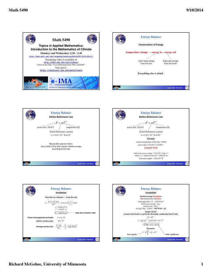
Math 5490 9/10/2014 Richard McGehee, University of Minnesota 1

Topics in Applied Mathematics: Introduction to the Mathematics of Climate

Mondays and Wednesdays 2:30 – 3:45

http://www.math.umn.edu/~mcgehee/teaching/Math5490-2014-2Fall/

Streaming video is available at

http://www.ima.umn.edu/videos/

Click on the link: "Live Streaming from 305 Lind Hall". Participation:

https://umconnect.umn.edu/mathclimate

Math 5490

Energy Balance

Conservation of Energy temperature change ~ energy in – energy out

short wave energy from the Sun long wave energy from the Earth

Everything else is detail.

Math 5490 9/10/2014

Energy Balance

Stefan‐Boltzmann Law

4

F T  

power flux (W/m2) temperature (K) Stefan-Boltzmann constant

8 2 4

5.67 10 W/m K 



 

Math 5490 9/10/2014

Reasonable approximation: Every body in the solar system radiates energy according to this law.

Energy Balance

Stefan‐Boltzmann Law

4

F T  

power flux (W/m2) temperature (K) Stefan-Boltzmann constant

8 2 4

5.67 10 W/m K 



  Example surface temperature of the Sun: 5780K power flux: 5.67x10-8 x (5780)4 = 6.33x107 W/m2 total solar power output: 6.33x107 x 4π(rS)2 , where rS = radius of the sun = 6.96x108 m total solar output: 3.85x1026 W

Math 5490 9/10/2014

Energy Balance

Insolation

Solar flux at a distance r from the sun:

2 7 2 7 2 2

6.33 10 4 6.33 10 W/m 4

S S

r r F r r             rS = 6.96x108 m r = 1.5x1011 m

2

1368 W/m F 

2 W E

F r   Power intercepted by the Earth: Math 5490 9/10/2014 solar flux at Earth’s orbit Earth’s surface area:

2 2

4 m

E

r  Average surface flux:

2 2 2

342 W/m 4 4

E E

F r F r     

Energy Balance

Insolation

Simple Model Assume that Earth is a perfectly thermally conducting black body. Global Average Insolation (Incoming solar radiation) intercepted flux: F = 1368 W/m2 Earth cross-section: πrE

2

surface area: 4πrE

2

average flux: 1368/4 = 342 W/m2 = Q

 

 

4 1 4 1 4 8

342 5.67 10 279K 6 C 43 F Q T T Q  



      

 

Dynamics

4

dT R Q T dt    heat capacity stable equilibrium Math 5490 9/10/2014

SLIDE 2

Math 5490 9/10/2014 Richard McGehee, University of Minnesota 2

Energy Balance

Goldilocks Zone

Solar flux at a distance r from the Sun:

2 7 2 7 2 2

6.33 10 4 6.33 10 W/m 4

S S

r r F r r             rS = 6.96x108 m

25 2 2

3.07 10 W/m F r   Average surface flux:

25 24 2 2 2

3.07 10 7.67 10 = W/m 4r r   Black body temperature:

24 4 2 2 1 4 24 8 2

7.67 10 = W/m 7.67 10 1.078 10 T r T r r              Math 5490 9/10/2014

Energy Balance

Goldilocks Zone

‐250 ‐200 ‐150 ‐100 ‐50 50 100 150 200 250 0.00 0.20 0.40 0.60 0.80 1.00 1.20 1.40 1.60 temperature (Celsius) distance from Sun (Tm) T(r) Mercury Earth Saturn

Math 5490 9/10/2014

Energy Balance

Goldilocks Zone

‐100 ‐50 50 100 150 0.00 0.05 0.10 0.15 0.20 0.25 0.30 temperature (Celsius) distance from Sun (Tm) T(r) Venus Earth Mars

Math 5490 9/10/2014

Energy Balance

Historical Overview of Climate Change Science, IPCC AR4, p.96

http://ipcc-wg1.ucar.edu/wg1/Report/AR4WG1_Print_CH01.pdf

albedo insolation OLR

Math 5490 9/10/2014

Energy Balance

Insolation

Simple Model Assume that Earth is a perfectly thermally conducting black body. Global Average Insolation (Incoming solar radiation) intercepted flux: F = 1368 W/m2 Earth cross-section: πrE

2

surface area: 4πrE

2

average flux: 1368/4 = 342 W/m2 = Q

 

 

4 1 4 1 4 8

342 5.67 10 279K 6 C 43 F Q T T Q  



      

 

Dynamics

4

dT R Q T dt    heat capacity stable equilibrium Math 5490 9/10/2014

Energy Balance

Historical Overview of Climate Change Science, IPCC AR4, p.96

http://ipcc-wg1.ucar.edu/wg1/Report/AR4WG1_Print_CH01.pdf

albedo insolation OLR

Math 5490 9/10/2014

SLIDE 3

Math 5490 9/10/2014 Richard McGehee, University of Minnesota 3

Energy Balance

Albedo

Not all the insolation reaches the surface. Some is reflected back into space. The proportion reflected is called the albedo, denoted α . For Earth, α ≈ 0.3 .

 

 

1 4 1 4 8

0.7 0.7 342 5.67 10 255K 18 C 0 F T F 



        

 

Simple Model Assume that Earth is a perfectly thermally conducting black body, but only 70% of the insolation is absorbed. Dynamics

4

(1 ) dT R Q T dt      stable equilibrium Math 5490 9/10/2014

Energy Balance

Historical Overview of Climate Change Science, IPCC AR4, p.96

http://ipcc-wg1.ucar.edu/wg1/Report/AR4WG1_Print_CH01.pdf

albedo insolation OLR

Math 5490 9/10/2014 Math 5490 9/10/2014

Energy Balance

OLR as a Function of Surface Temperature (Outgoing Longwave Radiation) OLR A BT  

A and B are determined from satellite observations. T is surface temperature (in Celsius).

4

(1 ) dT R Q T dt     

2 2

202 W/m 1.90 W/m K A B   Dynamics (1 ) ( ) dT R Q A BT dt      becomes photosphere temperature global mean surface temperature Kelvin Celsius

Energy Balance

OLR as a Function of Surface Temperature OLR A BT  

Important: A+BT is not a linear approximation to the Stefan- Boltzmann equation.

4

(1 ) dT R Q T dt      Dynamics (1 ) ( ) dT R Q A BT dt      becomes photosphere temperature global mean surface temperature Kelvin Celsius

different

Math 5490 9/10/2014

Energy Balance

Homogeneous Earth

(1 ) ( ) dT R Q A BT dt      Equilibrium Temperature:

 

1

eq

Q A BT      Stable, since B > 0 . Ice-free planet: α = 0.32, Teq = 16 °C Snowball planet: α = 0.62, Teq = -38 °C No glacier would form on an ice-free Earth. No glacier would melt on a snowball Earth. Easy question: Why do we have ice caps? Hard question: If Earth was ever a snowball, how did we get out?

 

1

eq

Q A T B     Math 5490 9/10/2014

Energy Balance

Latitude Dependence

 

( , ) ( )(1 ) ( , ) T y t R Qs y A BT y t t        Make T depend on y = sin(latitude) insolation distribution

 

2 2 2 2

2 ( ) 1 1 sin cos cos s y y y d



           

 

2 1

global annual average insolation 342W/m ( ) distribution across latitudes ( ) 1 Q s y s y dy    



One can show that

β = obliquity = 23.5°

Chylek and Coakley’s quadratic approximation:  

 

2

1 0.241 3 1 s y y    Math 5490 9/10/2014

SLIDE 4

Math 5490 9/10/2014 Richard McGehee, University of Minnesota 4

Insolation Distribution

0.1 0.2 0.3 0.4 0.5 0.6 0.7 0.8 0.9 1 0.5 0.6 0.7 0.8 0.9 1 1.1 1.2 1.3 sine(latitude) relative insolation approx today

green = quadratic approximation (Chylek & Coakley) fuchsia = formula using obliquity of 23.5°

Energy Balance

Math 5490 9/10/2014

Energy Balance

Latitude Dependence

 

( , ) ( )(1 ) ( , ) T y t R Qs y A BT y t t        Note that y is just a parameter. Equilibrium Temperature Profile ( )(1 ) ( )

eq

Qs y A T y B    

‐80 ‐60 ‐40 ‐20 20 40 60 0.2 0.4 0.6 0.8 1 temperature (Celsius) sin(latitude) ice free snowball

α = 0.32: ice free α = 0.62: snowball

Math 5490 9/10/2014

Energy Balance

Latitude Dependence

‐80 ‐60 ‐40 ‐20 20 40 60 0.2 0.4 0.6 0.8 1 temperature (Celsius) sin(latitude) ice free snowball

ice will form (icecap) ice won’t melt (no exit from snowball)

Math 5490 9/10/2014

Energy Balance

What’s Missing?

 

( , ) ( )(1 ) ( , ) T y t R Qs y A BT y t t        Math 5490 9/10/2014

Energy Balance

What’s Missing?

Math 5490 9/10/2014

Energy Balance

What’s Missing?

Math 5490 9/10/2014

SLIDE 5

Math 5490 9/10/2014 Richard McGehee, University of Minnesota 5

Energy Balance

What’s Missing?

Math 5490 9/10/2014

Energy Balance

What’s Missing?

Math 5490 9/10/2014

Energy Balance

What’s Missing?

Math 5490 9/10/2014

Energy Balance

What’s Missing? Weather!

Math 5490 9/10/2014

Energy Balance

Budyko’s Model

( )(1 ) ( ) ( ) T R Qs y A BT C T T t          Weather

1

( ) ( , ) T t T y t dt   Second Law of Thermodynamics: Energy travels from hot places to cold places. Budyko’s equation as a dynamical system: T lives in a function space (temperature as a function of latitude). Math 5490 9/10/2014 global mean temperature

Budyko’s Model

Why y ?

( , ) ( )(1 ) ( ( , )) ( ( ) ( , )) T y t R Qs y A BT y t C T t T y t t         

1

( ) ( , ) T t T y t dt  

Why do we use y = sine(latitude) instead of just latitude?

Math 5490 9/10/2014

global mean temperature:

SLIDE 6

Math 5490 9/10/2014 Richard McGehee, University of Minnesota 6

Why y ?

( , ) ( )(1 ) ( ( , )) ( ( ) ( , )) T y t R Qs y A BT y t C T t T y t t         

Why do we use y = sine(latitude) instead of just latitude?

Math 5490 9/10/2014

global mean temperature

Because y is directly proportional to surface area.

Budyko’s Model

1

( ) ( , ) T t T y t dt   http://mathworld.wolfram.com/ArchimedesHat-BoxTheorem.html

Why y = sine(latitude)?

θ h latitude h=sin(θ)

Math 5490 9/10/2014

Archimedes

Budyko’s Model

Why y = sine(latitude)?

Math 5490 9/10/2014

θ dθ cosθ

2 2 2 22 cos

2 sin 4 d

   

     

 

 



surface area of a unit sphere average over the sphere of a function of latitude f(θ)

1 1

1 ( ) 2 T T y dy



  ( substitute y = sin(θ) ) average over the sphere of a function T(y)

2 2 2 2 1 1

1 1 ( )2 cos ( )cos 4 2 1 (arcsin ) 2 f d f d f y dy

   

       

  

 

  

if T is symmetric across the equator:

1

( ) T T y dy  

Budyko’s Model

Why y = sine(latitude)?

Math 5490 9/10/2014

Budyko’s Model

0.1 0.2 0.3 0.4 0.5 0.6 0.7 0.8 0.9 1 10 20 30 40 50 60 70 80 90 surface area proportion latitude

Tropic of Cancer Minneapolis Arctic Circle

Budyko’s Equation ( )(1 ( )) ( ) ( ) T R Qs y y A BT C T T t         

heat transport OLR albedo insolation heat capacity surface temperature sin(latitude)

1

( ) T T y dy  

Budyko’s Model

sin(latitude) 1 y    Symmetry assumption: Chylek and Coakley’s quadratic approximation:  

 

2

1 0.241 3 1 s y y   

Math 5490 9/10/2014