Math 5490 9/22/2014 Energy Balance Math 5490 Dynamical Models - - PDF document

SLIDE 1

Math 5490 9/22/2014 Richard McGehee, University of Minnesota 1

Topics in Applied Mathematics: Introduction to the Mathematics of Climate

Mondays and Wednesdays 2:30 – 3:45

http://www.math.umn.edu/~mcgehee/teaching/Math5490-2014-2Fall/

Streaming video is available at

http://www.ima.umn.edu/videos/

Click on the link: "Live Streaming from 305 Lind Hall". Participation:

https://umconnect.umn.edu/mathclimate

Math 5490

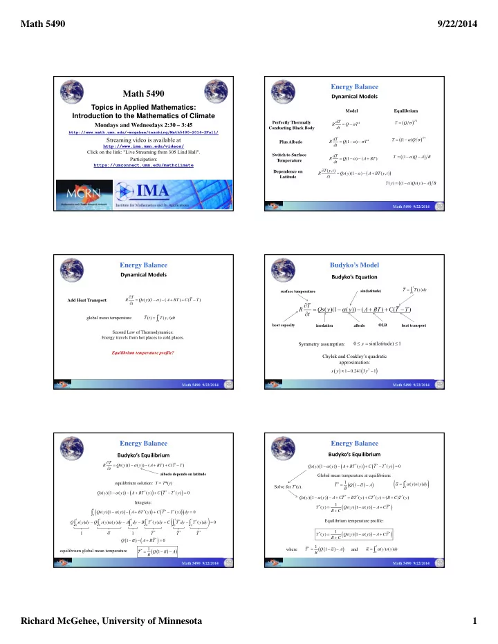
Energy Balance

Dynamical Models

Perfectly Thermally Conducting Black Body

4

dT R Q T dt    Math 5490 9/22/2014

4

(1 ) dT R Q T dt      (1 ) ( ) dT R Q A BT dt      Plus Albedo Switch to Surface Temperature

 

( , ) ( )(1 ) ( , ) T y t R Qs y A BT y t t        Dependence on Latitude

 

1 4

T Q  

 

1 4

(1 ) T Q    

 

(1 ) T Q A B    

 

( ) (1 ) ( ) T y Qs y A B     Model Equilibrium

Energy Balance

( )(1 ) ( ) ( ) T R Qs y A BT C T T t         

1

( ) ( , ) T t T y t dt   Second Law of Thermodynamics: Energy travels from hot places to cold places. Equilibrium temperature profile? global mean temperature

Dynamical Models

Add Heat Transport

Math 5490 9/22/2014

Budyko’s Equation ( )(1 ( )) ( ) ( ) T R Qs y y A BT C T T t         

heat transport OLR albedo insolation heat capacity surface temperature sin(latitude)

1

( ) T T y dy  

Budyko’s Model

sin(latitude) 1 y    Symmetry assumption: Chylek and Coakley’s quadratic approximation:  

 

2

1 0.241 3 1 s y y   

Math 5490 9/22/2014

Energy Balance

Budyko’s Equilibrium

( )(1 ( )) ( ) ( ) T R Qs y y A BT C T T t          equilibrium solution: T = T*(y)

  

  

* * *

( ) 1 ( ) ( ) ( ) Qs y y A BT y C T T y        Integrate:

  

    

 

1 * * * 1 1 1 1 1 1 * * *

( ) 1 ( ) ( ) ( ) ( ) ( ) ( ) ( ) ( ) Qs y y A BT y C T T y dy Q s y dy Q s y y dy A dy B T y dy C T dy T y dy              

      

 albedo depends on latitude

*

T

*

T

*

T 1 1

  



*

1 Q A BT     

   

*

1 1 T Q A B     equilibrium global mean temperature Math 5490 9/22/2014

Energy Balance

Budyko’s Equilibrium

 

1

( ) ( ) y s y dy    

   

*

1 1 T Q A B     Global mean temperature at equilibrium:

  

  

* * *

( ) 1 ( ) ( ) ( ) Qs y y A BT y C T T y        Equilibrium temperature profile:

   

 

* * * * * *

( ) 1 ( ) ( ) ( ) ( ) ( ) 1 ( ) ( ) 1 ( ) Qs y y A CT BT y CT y B C T y T y Qs y y A CT B C               Solve for T*(y).

 

 

* *

1 ( ) ( ) 1 ( ) T y Qs y y A CT B C      

   

*

1 1 T Q A B    

1

( ) ( ) y s y dy     where and Math 5490 9/22/2014

SLIDE 2

Math 5490 9/22/2014 Richard McGehee, University of Minnesota 2

Energy Balance

Budyko’s Equilibrium

  

  

* * *

( ) 1 ( ) ( ) ( ) Qs y y A BT y C T T y        Equilibrium temperature profile:

‐80 ‐60 ‐40 ‐20 20 40 60 0.2 0.4 0.6 0.8 1 temperature (Celsius) sin(latitude) ice free snowball ice free (C=0) snowball (C=0)

 

 

* *

1 ( ) ( ) 1 ( ) T y Qs y y A CT B C       C = 3.04 α(y) = 0.32: ice free α(y) = 0.62: snowball (constant albedo) Math 5490 9/22/2014

Energy Balance

Budyko’s Equilibrium

‐80 ‐60 ‐40 ‐20 20 40 60 0.2 0.4 0.6 0.8 1 temperature (Celsius) sin(latitude) ice free snowball ice free (C=0) snowball (C=0)

ice won’t melt (no exit from snowball) ice will form (icecap)

Math 5490 9/22/2014

http://www.i-fink.com/melting-polar-ice/

Budyko’s Model

Ice Albedo Feedback temperature warms ice melts albedo decreases more sunlight absorbed temperature warms REPEAT Why would it stop?

Math 5490 9/22/2014

Budyko’s Model

Ice Albedo Feedback temperature warms ice melts albedo decreases more sunlight absorbed temperature warms REPEAT Why would it stop?

• M. I. Budyko, "The effect of solar radiation

variations on the climate of the Earth," Tellus XXI, 611-619 , 1969.

http://www.inenco.org/index_principals.html

Math 5490 9/22/2014

Budyko’s Equation ( )(1 ( )) ( ) ( ) T R Qs y y A BT C T T t         

heat transport OLR albedo insolation heat capacity surface temperature sin(latitude)

1

( ) T T y dy  

Budyko’s Model

Math 5490 9/22/2014

Ice Albedo Feedback Why would it stop?

Budyko’s Model

Ice Albedo Feedback

What if the albedo is not constant? Ice Line Assumption: There is a single ice line at y=η between the equator and the pole. The albedo is α1 below the ice line and α2 above it.

1 2

( , ) and y y y             Equilibrium condition:

  

  

* * *

( ) 1 ( , ) ( ) ( ) Qs y y A BT y C T T y

 

       

 

 

* *

1 ( ) ( ) 1 ( , ) T y Qs y y A CT B C

 

      

   

*

1 1 ( ) T Q A B



    

 

1

( ) ( , ) ( ) y s y dy       Equilibrium solution: where Math 5490 9/22/2014

SLIDE 3

Math 5490 9/22/2014 Richard McGehee, University of Minnesota 3

Budyko’s Model

Ice Albedo Feedback

1 2

0.32, ( , ) 0.62, y y y              

 

 

   

* * *

1 1 ( ) ( ) 1 ( , ) , where 1 ( ) T y Qs y y A CT T Q A B C B

  

           

1 1 1 2

( ) ( , ) ( ) ( ) ( ) y s y dy s y dy s y dy

 

        

  

1 1

( ) ( ) , 1 ( ) ( ) , since 1 ( ) S s y dy S s y dy s y dy

 

     

  

equilibrium temperature profile: albedo:

1 2 2 2 1

( ) ( ) (1 ( )) ( ) ( ) 0.62 0.3 ( ) S S S S                    global albedo: let: then: Math 5490 9/22/2014

     

2 3

( ) ( ) 1 0.241 3 1 0.241 S s y dy y dy

 

          

 

Chylek & Coakley

Budyko’s Model

Ice Albedo Feedback

1 2

0.32, ( , ) 0.62, y y y              

 

 

   

* * *

1 1 ( ) ( ) 1 ( , ) , where 1 ( ) T y Qs y y A CT T Q A B C B

  

           

1 1 1 2

( ) ( , ) ( ) ( ) ( ) y s y dy s y dy s y dy

 

        

  

1 1

( ) ( ) , 1 ( ) ( ) , since 1 ( ) S s y dy S s y dy s y dy

 

     

  

equilibrium temperature profile: albedo:

1 2 2 2 1

( ) ( ) (1 ( )) ( ) ( ) 0.62 0.3 ( ) S S S S                    global albedo: let: then: Math 5490 9/22/2014

     

2 3

( ) ( ) 1 0.241 3 1 0.241 S s y dy y dy

 

          

 

Chylek & Coakley

Budyko’s Model

Ice Albedo Feedback

For each fixed η , there is an equilibrium solution for Budyko’s equation.

 

 

* *

1 ( ) ( ) 1 ( , ) T y Qs y y A CT B C

 

      

‐50 ‐40 ‐30 ‐20 ‐10 10 20 30 0.1 0.2 0.3 0.4 0.5 0.6 0.7 0.8 0.9 1 °C sine(latitude)

45° 23.5° 66.5° Math 5490 9/22/2014

Budyko’s Model

Dynamics

Let X be the space of functions where T lives. (e.g. L1([0,1]) ) Let

 

: : ( ) , ( ) ( ) 1 ( ) L X X LT CT B C T f y Qs y y A         dT R f LT dt   Budyko’s equation can be written as a linear vector field on X . ( )(1 ( )) ( ) ( ) T R Qs y y A BT C T T t          The operator L has only point spectrum, with all eigenvalues negative. Therefore, all solutions are stable. True for any albedo function. Math 5490 9/22/2014

experts only

Budyko’s Model

Ice Albedo Feedback

‐50 ‐40 ‐30 ‐20 ‐10 10 20 30 0.1 0.2 0.3 0.4 0.5 0.6 0.7 0.8 0.9 1 °C sine(latitude)

45° 23.5° 66.5°

For each fixed η , there is a globally stable equilibrium solution for Budyko’s equation. How to pick one? ( )(1 ( , )) ( ) ( ) T R Qs y y A BT C T T t          

Math 5490 9/22/2014

Budyko’s Model

Ice Albedo Feedback Summary If we artificially hold the ice line at a fixed latitude, then the surface temperature will come to an equilibrium. However, if the temperature is high, we would expect ice to melt and the ice line to retreat to higher latitudes. If the temperature is low, we would expect ice to form and the ice line to advance to lower latitudes. How to model this expectation?

Math 5490 9/22/2014

SLIDE 4

Math 5490 9/22/2014 Richard McGehee, University of Minnesota 4

Budyko’s Model

Ice Albedo Feedback

For each fixed η , there is a stable equilibrium solution for Budyko’s equation. Standard assumption: Permanent ice forms if the annual average temperature is below Tc=-10 °C and melts if the annual average temperature is above Tc. Additional condition: The average temperature across the ice boundary is the critical temperature Tc .

‐50 ‐40 ‐30 ‐20 ‐10 10 20 30 0.0 0.2 0.4 0.6 0.8 1.0 T(y) y ‐50 ‐40 ‐30 ‐20 ‐10 10 20 30 0.0 0.2 0.4 0.6 0.8 1.0 T(y) y ‐50 ‐40 ‐30 ‐20 ‐10 10 20 30 0.0 0.2 0.4 0.6 0.8 1.0 T(y) y

looks okay looks okay not good

+ + +

 

* *

1 ( ) ( ) 10 2

c

T T T

 

       

Math 5490 9/22/2014

Budyko’s Model

Ice Albedo Feedback

 

* *

1 ( ) ( ) 10 2

c

T T T

 

       

Math 5490 9/22/2014

ice line condition:

‐50 ‐40 ‐30 ‐20 ‐10 10 20 30 0.0 0.2 0.4 0.6 0.8 1.0 T(y) y

η Tη

* (η+)

Tη

* (η−)

Budyko’s Model

Ice Albedo Feedback

( )(1 ( , )) ( ) ( ) T R Qs y y A BT C T T t           Ice line condition:

 

* *

1 ( ) ( ) 10 2

c

T T T

 

        where: Math 5490 9/22/2014

 

 

* *

1 ( ) ( ) 1 ( , ) T y Qs y y A CT B C

 

      

1 2

0.32, ( , ) 0.62, y y y              

1 2

( , ) , ( , )            

1 2

0.47 2      

 

 

* * 2

1 ( ) ( ) 1 T Qs A CT B C

 

        

 

 

* * 1

1 ( ) ( ) 1 T Qs A CT B C

 

         Equilibrium: Albedo:

 

 

 

* * *

1 1 ( ) ( ) ( ) 1 10 2

c

T T Qs A CT T B C

  

               Ice line condition:

Budyko’s Model

Ice Albedo Feedback

( )(1 ( , )) ( ) ( ) T R Qs y y A BT C T T t           Ice line condition: where: Math 5490 9/22/2014 Recall equilibrium GMT: Recall average albedo:

 

 

*

1 ( ) 1 10

c

Qs A CT T B C



        

   

*

1 1 ( ) T Q A B



    

1 2 2 1

( ) ( , ) ( ) ( ) ( ) 0.62 0.3 ( ) y s y dy S S               



 

3

( ) ( ) 0.241 S s y dy



       



 

 

*

1 ( ) ( ) 1

c

h Qs A CT T B C



          Rewrite:

        

2 2 1

1 1 ( )

c

Q C A h s S T B C B B                       

Budyko’s Model

Ice Albedo Feedback

( )(1 ( , )) ( ) ( ) T R Qs y y A BT C T T t           The additional condition:

 

* *

1 ( ) ( ) 10 2

c

T T T

 

       

        

2 2 1

1 1 ( )

c

Q C A h s S T B C B B                        Two equilibria (zeros

• f h ) satisfy the

additional condition.

‐10 ‐8 ‐6 ‐4 ‐2 2 4 6 0.1 0.2 0.3 0.4 0.5 0.6 0.7 0.8 0.9 1

h(η) η

can be written:

Math 5490 9/22/2014

Budyko’s Model

Ice Albedo Feedback

• 50
• 40
• 30
• 20
• 10

10 20 30 0.0 0.2 0.4 0.6 0.8 1.0 temperature (ºC) sin(latitude) ice free snowball small cap big cap

Interesting Solutions: small cap large cap ice free snowball

Math 5490 9/22/2014

 

 

* *

1 ( ) ( ) 1 ( , ) T y Qs y y A CT B C

 

       Equilibrium temperature profiles

SLIDE 5

Math 5490 9/22/2014 Richard McGehee, University of Minnesota 5

Budyko’s Model

Dynamics of the Ice Line

( )(1 ( , )) ( ) ( ) T R Qs y y A BT C T T t          

‐50 ‐40 ‐30 ‐20 ‐10 10 20 30 0.0 0.2 0.4 0.6 0.8 1.0 T(y) y ‐50 ‐40 ‐30 ‐20 ‐10 10 20 30 0.0 0.2 0.4 0.6 0.8 1.0 T(y) y ‐50 ‐40 ‐30 ‐20 ‐10 10 20 30 0.0 0.2 0.4 0.6 0.8 1.0 T(y) y

stationary stationary ice melts

+ + +

Idea: If the average temperature across the ice line is above the critical temperature, some ice will melt, moving the ice line toward the pole. If it is below the critical temperature, the ice will advance toward the equator.

 

( )

c

d T T dt      Widiasih’s equation:

Math 5490 9/22/2014

Budyko’s Model

 

( ) ( )(1 ( , )) ( ) ( )

c

d T T dt T R Qs y y A BT C T T t                State space: [0,1]

X 

‐10 ‐8 ‐6 ‐4 ‐2 2 4 6 0.1 0.2 0.3 0.4 0.5 0.6 0.7 0.8 0.9 1

h(η) η stable unstable

Dynamics of the Ice Line

Math 5490 9/22/2014

( ) d h dt     Widiasih’s Theorem. For sufficiently small ε , the system has an attracting invariant curve given by the graph of a function Φε : [0,1] → X . On this curve, the dynamics are approximated by the equation

experts only

Esther R. Widiasih, Dynamics of the Budyko Energy Balance Model, SIAM J. Appl. Dyn. Syst., 12(4), 2068–2092.

Budyko’s Model

Budyko‐Widiasih Model

 

d h dt    

0.1 0.2 0.3 0.4 0.5 0.6 0.7 0.8 0.9 1

• 60
• 50
• 40
• 30
• 20
• 10

10 20 30

Temperature profiles Math 5490 9/22/2014

Budyko’s Model

Summary ( )(1 ( )) ( ) ( ) T R Qs y y A BT C T T t         

heat transport OLR albedo insolation heat capacity surface temperature sin(latitude)

1

( ) T T y dy  

reduces to ( ) d h dt             

2 2 1

1 1 ( )

c

d Q C A h s S T dt B C B B                                 Math 5490 9/22/2014

Budyko’s Model

Budyko‐Widiasih Model What about the greenhouse effect?

A+BT is the outgoing long wave radiation. This term decreases if the greenhouse gases increase. We view A as a parameter.   , d h A dt    

( )(1 ( )) ( ) ( ) T R Qs y y A BT C T T t         

heat transport OLR albedo insolation heat capacity surface temperature sin(latitude)

1

( ) T T y dy   Math 5490 9/22/2014

Budyko’s Model

Budyko‐Widiasih Model

 

, d h A dt    

175 180 185 190 195 200 205 210 215 220 0.1 0.2 0.3 0.4 0.5 0.6 0.7 0.8 0.9 1

A  high CO2 low CO2 isocline

 

, h A   Math 5490 9/22/2014

SLIDE 6

Math 5490 9/22/2014 Richard McGehee, University of Minnesota 6

Snowball Earth

http://www.astrobio.net/topic/solar-system/earth/new-information-about- snowball-earth-period/

Math 5490 9/22/2014

Is it possible for Earth to become completely covered in ice? (Snowball Earth) Did it ever happen?

http://www.snowballearth.org/when.html

Math 5490 9/22/2014

Snowball Earth

There is evidence that Snowball Earth has

• ccurred, the last

time about 600 million years ago.

Hoffman & Schrag, Snowball Earth, SCIENTIFIC AMERICAN, January 2000, 68-75 Math 5490 9/22/2014

Snowball Earth

The continents were clustered near the equator.

Hoffman & Schrag, Snowball Earth, SCIENTIFIC AMERICAN, January 2000, 68-75 Math 5490 9/22/2014

Snowball Earth

“Ice‐rafted debris” occurred in ocean sediments near the equator, indicating large equatorial glaciers calving icebergs.

Hoffman & Schrag, Snowball Earth, SCIENTIFIC AMERICAN, January 2000, 68-75 Math 5490 9/22/2014

Snowball Earth

Large limestone deposits “cap carbonates” are found immediately above the glacial debris, indicating a rapid warming period following the snowball.

Math 5490 9/22/2014

Snowball Earth

Idea: When the Earth is mostly ice‐covered, silicate weathering slows down, but volcanic activity stays the same, allowing for a build‐up of CO2 in the atmosphere. When the Earth is mostly ice‐free, silicate weathering speeds up, drawing down the CO2 in the atmosphere.

SLIDE 7

Math 5490 9/22/2014 Richard McGehee, University of Minnesota 7

Budyko’s Model

Budyko‐Widiasih Model

 

, d h A dt    

What if A is a dynamical variable?  

c

dA dt       1      

   

,

c

dA dt d h A dt           Simple equation: New system: MCRN Paleocarbon equation (silicate weathering) Math 5490 9/22/2014

Budyko’s Model

Budyko‐Widiasih‐Paleocarbon Model

175 180 185 190 195 200 205 210 215 220 0.1 0.2 0.3 0.4 0.5 0.6 0.7 0.8 0.9 1

A  high CO2 low CO2

c



stable rest point

   

, ,

c

d dA h A dt dt           What if ηc were here?

Math 5490 9/22/2014

Budyko’s Model

Budyko‐Widiasih‐Paleocarbon Model

   

, ,

c

d dA h A dt dt          

175 180 185 190 195 200 205 210 215 220 0.1 0.2 0.3 0.4 0.5 0.6 0.7 0.8 0.9 1

A 

c



unstable rest point

What if ηc were here?

high CO2 low CO2 Math 5490 9/22/2014

Budyko’s Model

Snowball – Hothouse Oscillations

175 180 185 190 195 200 205 210 215 220 0.1 0.2 0.3 0.4 0.5 0.6 0.7 0.8 0.9 1

A 

c

 high CO2 low CO2

Budyko‐Widiasih‐Paleocarbon Model

Math 5490 9/22/2014

Budyko’s Model

Suggested Reading

Math 5490 9/22/2014

Hoffman & Schrag, Snowball Earth, SCIENTIFIC AMERICAN, January 2000, 68-75 K.K. Tung, Topics in Mathematical Modeling, PRINCETON UNIVERSITY PRESS, 2007, Chapter 8