SLIDE 2 Math 5490 11/17/2014 Richard McGehee, University of Minnesota 2
Dynamical Systems
Math 5490 11/17/2014
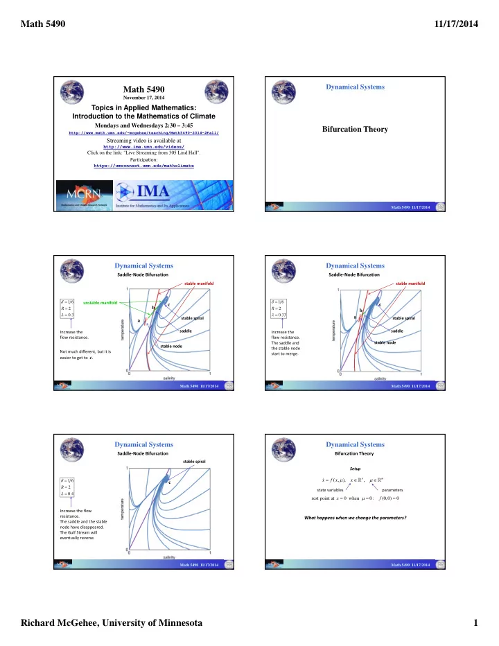
Bifurcation Theory ( , ), ,
n m
x f x x
No Bifurcation (Poincaré Continuation) rest point at 0 when 0 : (0,0) x f
1
The Jacobian matrix (0,0) is nonsingular, i.e., has no zero eigenvalues. D f Conclusion For small values of , there is a rest point ( ) satisfying (0) 0, ( ( ), ) 0. p p f p The rest point “continues” for small parameter values.
Dynamical Systems
Math 5490 11/17/2014
Bifurcation Theory ( , ), ,
n m
x f x x
Poincaré Continuation rest point at 0 when 0 : (0,0) x f
2 1 1 2
We can write ( , ) O ( , ) 0, where (0,0) and is an matrix and solve for : ( ) O ( ). f x Ax B x A D f B n m x x p A B
Idea of Proof
1
If Jacobian matrix (0,0) is nonsingular, then, for small values of , there is a rest point ( ) satisfying (0) 0, ( ( ), ) 0. D f p p f p
Dynamical Systems
Math 5490 11/17/2014
Bifurcation Theory ( , ), ,
n m
x f x x
rest point at 0 when 0: (0,0) x f There’s more!
1 1
If is continuously differentiable ( ), then the Jacobian matrix ( ( ), ) varies continuously with , as do the eigenvalues and eigenvectors. f C D f p If the rest point at μ = 0 is hyperbolic (or a saddle, or a stable node,
- r an unstable node, or a stable spiral, or an unstable spiral), then the
rest point p(μ ) inherits the property for small values of μ . Poincaré Continuation
1
If Jacobian matrix (0,0) is nonsingular, then, for small values of , there is a rest point ( ) satisfying (0) 0, ( ( ), ) 0. D f p p f p
Dynamical Systems
Classification
determinant trace Math 5490 11/17/2014
Poincare continuation Poincare continuation fails when determinant = 0.
Kaper & Engler, 2013
Dynamical Systems
Math 5490 11/17/2014
Bifurcation Theory
Example
2
In this example, we can solve explicitly: 2 2 4 4 1 1 . 2 Since (0) 0 , we take the "+" sign: ( ) 1 1 . x x x p x p
2 1 1 2
( , ) 2 ( , ) 2 2 , so (0,0) 2 0, so there is a rest point ( ) satisfying (0) 0. ( ) O ( ). 2 x f x x x D f x x D f x p p x p For each value of μ close to 0, there is a unique rest point near x = 0.
Dynamical Systems
Bifurcation Theory
Example
1
Note that there is another rest point at 2 for 0. Its eigenvalue is ( 2,0) 2 2( 2) 2, so it is unstable. Futhermore, for small values of , there is a unique rest point ( ) near 2, x D f p x and that rest point is unstable.
2 1 1
( , ) 2 ( , ) 2 2 , so (0,0) 2, so the rest point ( ) has an eigenvalue near 2 for small and hence is asymptotically stable. x f x x x D f x x D f x p 2 small Math 5490 11/17/2014