Math 5490 11/10/2014 Dynamical Systems Math 5490 Nonlinear Systems - - PDF document

SLIDE 1

Math 5490 11/10/2014 Richard McGehee, University of Minnesota 1

Topics in Applied Mathematics: Introduction to the Mathematics of Climate

Mondays and Wednesdays 2:30 – 3:45

http://www.math.umn.edu/~mcgehee/teaching/Math5490-2014-2Fall/

Streaming video is available at

http://www.ima.umn.edu/videos/

Click on the link: "Live Streaming from 305 Lind Hall". Participation:

https://umconnect.umn.edu/mathclimate

Math 5490

November 10, 2014

Dynamical Systems

Math 5490 11/10/2014

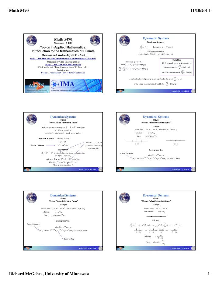
Nonlinear Systems

If is small, i.e., if is close to , then solutions of ( ) are close to solutions of ( ) . x p d f p dt d Df p dt         Rest point : ( ) p f p  ( ) dx f x dt  Introduce . Then ( ) ( ) ( ) ( ) ( ) ( ) x p f x f p Df p d dx f x f p Df p dt dt                 Basic Idea Linear approximation: ( ) ( ) ( )( ) ( )( ) f x f p Df p x p Df p x p      In particular, the rest point is asymptotically stable for ( ) if the origin is asymptotically stable for ( ) . dx p f x dt d Df p dt    

Dynamical Systems

Math 5490 11/10/2014

Flows “Vector Fields Determine Flows”

A is a continuous map : satisfying ( ,0) , for all , ( , ) ( ( , ), ), for all , , and .

n n

flow x x x x t s x t s x t s              ( ) ( , ) id

t t s t s

x x t      



    Alternate Notation Big Theorem If : is smooth, then the initial value problem ( ), (0) , defines a flow : satisfying ( , ) ( ( , )), ( ,0) . Also, is a smooth as .

n n n n

f x f x x x x t f x t x x f                     : , ( times continuously differentiable)

n

Smooth C n n  Group Property

Dynamical Systems

Math 5490 11/10/2014

Flows “Vector Fields Determine Flows”

vector field: , , initial value: (0) solution: flow: ( , )

at at

x ax x x x x e x x t e x         Example     Check properties:

( )

( ,0) ( , ) ( , ) ( ( , ), )

a a t s at as at

x e x x x t s e x e e x e x s x s t     

 

       Group Property

Dynamical Systems

Math 5490 11/10/2014

Flows “Vector Fields Determine Flows”

vector field: , initial value: (0) solution: flow: ( , )

n tA tA

x Ax x x x x e x x t e x         Example Check properties:

( )

( ,0) ( , ) ( , ) ( ( , ), )

A t s A tA sA tA

x e x x x t s e x e e x e x s x s t     

 

       Group Property Experts Only

Dynamical Systems

Math 5490 11/10/2014

Flows “Vector Fields Determine Flows”

2

vector field: , initial value: (0) x x x x x      Example

2 2 2 1

1 1 1 1 1 1

x x t x x

dx x x dx dt x dx dt x t dt x t x t t x x x x x x x t

  

                  

 

Calculus solution: 1 flow: ( , ) 1 x x x t x x t x t     

SLIDE 2

Math 5490 11/10/2014 Richard McGehee, University of Minnesota 2

Dynamical Systems

Math 5490 11/10/2014

Flows “Vector Fields Determine Flows”

2

vector field: , initial value: (0) flow: ( , ) 1 x x x x x x x t x t         Example group property Check properties: ( ,0) 1 ( , ) 1 ( ( , ), ) ( , ) 1 ( , ) 1 1 ( ) 1 1 x x x x x x t x x x t x t s x t s x x t s x t x s x t s s x t                        

Dynamical Systems

Math 5490 11/10/2014

Flows “Vector Fields Determine Flows”

2

vector field: , initial value: (0) flow: ( , ) 1 x x x x x x x t x t         Example Calculus Issue: Solutions do not exist for all time. 1 ( , ) as 1 x x t t x t x       local flow: Solutions exist for some time interval.

Dynamical Systems

Math 5490 11/10/2014

Flows “Vector Fields Determine Flows”

2

vector field: 1 , initial value: (0) x x x x x       Example

 

2 2 1 2 1 1 1 1 1 1 1 1 1

1 (1 ) (1 ) tanh tanh tanh tanh tanh tanh tanh tanh(tanh ) tanh tanh 1 tanh 1 tanh(tanh )tanh

x x t x x

dx x x dx dt x dx dt x t dt x x t x x t x x t x t x t x x t x t

         

                       

 

Calculus tanh flow: ( , ) 1 tanh x t x t x t    

Dynamical Systems

Math 5490 11/10/2014

Flows “Vector Fields Determine Flows”

2

vector field: 1 , initial value: (0) tanh flow: ( , ) 1 tanh x x x x x x t x t x t           Example Group Property tanh tanh tanh( ) tanh tanh tanh tanh 1 tanh tanh ( , ) tanh tanh 1 tanh( ) 1 tanh tanh (tanh tanh ) 1 1 tanh tanh t s x x t s x x t s t s t s x t s t s x t s t s x t s x t s                      tanh tanh ( , ) tanh tanh tanh tanh tanh 1 tanh ( ( , ), ) tanh 1 ( , )tanh 1 tanh tanh tanh tanh 1 tanh 1 tanh x t s x t t x t s x t s x t x t s x t x t t x t x s t s s x t                      equal

Dynamical Systems

Math 5490 11/10/2014

Flows “Vector Fields Determine Flows”

2

vector field: 1 , tanh flow: ( , ) 1 tanh x x x x t x t x t          local Example Issue: Solutions do not exist for all time.

1

tanh 1 ( , ) as tanh ( 1 ) 1 tanh x t x x t t x x t 



         

1

tanh 1 ( , ) as tanh ( 1 ) 1 tanh x t x x t t x x t 



         

Dynamical Systems

Math 5490 11/10/2014

Flows  

vector field: ( ), (0) , flow: ( , ) ( , )

n

x f x x x x x t f x t          Backwards Time

   

Let ( , ) ( , ) then ( , ) ( , ) ( , ) ( , ) ( , ) x t x t x t x t x t f x t f x t t t                         So ( ,t) satisfies ( ), (0) x x f x x x      Going backward in time is the same as following the negative of the vector field.

SLIDE 3

Math 5490 11/10/2014 Richard McGehee, University of Minnesota 3

Dynamical Systems

Math 5490 11/10/2014

Flows “Vector Fields Determine Flows”

2

vector field: 1 , tanh local flow: ( , ) 1 tanh x x x x t x t x t          Example

 

2

vector field: 1 , tanh local flow: ( , ) 1 tanh x x x x t x t x t           tanh tanh( ) ( , ) ( , ) 1 tanh 1 tanh( ) x t x t x t x t x t x t            

Dynamical Systems

Math 5490 11/10/2014

Nonlinear Systems

Rest point : ( ) p f p  ( ) dx f x dt  The rest point is called if it is stable and if there exists a 0 such that ( , ) as . p x p x t p t           asymptotically stable Stability

 

The rest point is called

• r simply

if, for all 0, there exists a 0 such that ( , ) for all 0. It is called if it is not stable. p x p x t p t              Lyapunov stable stable unstable

Dynamical Systems

Math 5490 11/10/2014

Nonlinear Systems

Stability unstable

Dynamical Systems

Math 5490 11/10/2014

Stability

Lyapunov stable asymptotically stable unstable

Dynamical Systems

Math 5490 11/10/2014

Nonlinear Systems

Rest point : ( ) p f p  ( ) dx f x dt  variational equation near : ( ) d p Df p dt    x p    Jacobian matrix If all of the eigenvalues of the Jacobian matrix have negative real part, then the rest point p is asymptotically stable. If any eigenvalue of the Jacobian matrix has positive real part, then the rest point p is unstable. If all of the eigenvalues of the Jacobian matrix have positive real part, then the rest point p is asymptotically stable for the backwards flow.

Dynamical Systems

Math 5490 11/10/2014

Nonlinear Systems

Rest point : ( ) p f p 

2

( ), dx f x x dt   What about saddles? If one of the eigenvalues of the Jacobian matrix is positive and the other is negative, then there are two smooth curves intersecting at , ( ) (the stable manifold), and ( ) (the unstable manif

s u

p W p W p

• ld) satisfying these properities:

( ) ( , ) as ( ) ( , ) as ( ) is tangent at to the eigenvector corresponding to the negative eigenvalue ( ) is tangent at to th

s u s u

x W p x t p t x W p x t p t W p p W p p             e eigenvector corresponding to the positive eigenvalue

SLIDE 4

Math 5490 11/10/2014 Richard McGehee, University of Minnesota 4

Dynamical Systems

Math 5490 11/10/2014

Nonlinear Systems

Rest point : ( ) p f p 

2

( ), dx f x x dt   What about saddles? stable manifold unstable manifold

Dynamical Systems

Nonlinear Systems

3

dx x x y dt dy y dt      Example Math 5490 11/10/2014 rest points: ( 1,0), (0,0), and (1,0) 

Dynamical Systems

Nonlinear Systems

Example

2

1 3 1 ( , ) 1 x Df x y         

3

dx x x y dt dy y dt      2 1 1 1 2 1 ( 1,0) (0,0) (1,0) 1 1 1 Df Df Df                            Math 5490 11/10/2014

Dynamical Systems

Nonlinear Systems

3

dx x x y dt dy y dt      Example Rest points: ( 1,0), (0,0), and (1,0)  2 1 1 1 2 1 ( 1,0) (0,0) (1,0) 1 1 1 Df Df Df                            Math 5490 11/10/2014 eigenvalues: 2 1 1 1 eigenvectors: 1               eigenvalues: 1 1 1 1 eigenvectors: 2               sinks saddle fast slow unstable stable

Dynamical Systems

Nonlinear Systems

1 1 , (0,0) 1 A A Df              Example Math 5490 11/10/2014 eigenvalues: 1 1 1 1 eigenvectors: 2               saddle

3

dx x x y dt dy y dt      stable unstable unstable stable

Dynamical Systems

Nonlinear Systems

1 1 , (0,0) 1 Ax A Df             Example Math 5490 11/10/2014 eigenvalues: 1 1 1 1 eigenvectors: 2               saddle

3

dx x x y dt dy y dt     

SLIDE 5

Math 5490 11/10/2014 Richard McGehee, University of Minnesota 5

Dynamical Systems

Nonlinear Systems

3

dx x x y dt dy y dt      Example Math 5490 11/10/2014 unstable stable

Dynamical Systems

Nonlinear Systems

2 1 , ( 1,0) (1,0) 1 A A Df Df                 Example Math 5490 11/10/2014 eigenvalues: 2 1 1 1 eigenvectors: 1               stable node

3

dx x x y dt dy y dt      slow fast slow fast

Dynamical Systems

Nonlinear Systems

2 1 , ( 1,0) (1,0) 1 A A Df Df                 Example Math 5490 11/10/2014 eigenvalues: 2 1 1 1 eigenvectors: 1               stable node

3

dx x x y dt dy y dt     

Dynamical Systems

Nonlinear Systems

3

dx x x y dt dy y dt      Example Math 5490 11/10/2014 fast slow unstable stable

Dynamical Systems

Nonlinear Systems

3

dx x x y dt dy y dt      Example Math 5490 11/10/2014 saddle stable manifold unstable manifold

Dynamical Systems

Nonlinear Systems

3

dx x x y dt dy y dt      Example Math 5490 11/10/2014 stable manifold unstable manifold slow direction fast direction

SLIDE 6

Math 5490 11/10/2014 Richard McGehee, University of Minnesota 6

Stommel’s Model

Stommel, TELLUS XII (1961)

stable spiral saddle stable node

Dynamical Systems

Math 5490 11/10/2014