Math 5490 11/12/2014 Dynamical Systems Math 5490 Stommels Model - - PDF document

▶

$math 5490 11 12 2014$

Jul 17, 2023 505 likes •596 views

Math 5490 11/12/2014 Dynamical Systems Math 5490 Stommels Model November 12, 2014 Topics in Applied Mathematics: Henry Stommel, Thermohaline Convection with Two Stable Regimes of Flow , T ELLUS XII (1961), 224-230. Introduction to the

SLIDE 1

Math 5490 11/12/2014 Richard McGehee, University of Minnesota 1

Topics in Applied Mathematics: Introduction to the Mathematics of Climate

Mondays and Wednesdays 2:30 – 3:45

http://www.math.umn.edu/~mcgehee/teaching/Math5490-2014-2Fall/

Streaming video is available at

http://www.ima.umn.edu/videos/

Click on the link: "Live Streaming from 305 Lind Hall". Participation:

https://umconnect.umn.edu/mathclimate

Math 5490

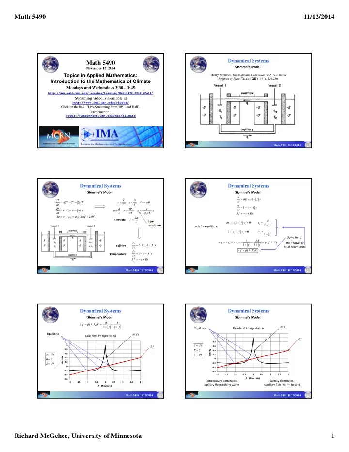
November 12, 2014 Stommel’s Model

Henry Stommel, Thermohaline Convection with Two Stable Regimes of Flow, TELLUS XII (1961), 224-230.

Dynamical Systems

Math 5490 11/12/2014

Stommel’s Model

(1 ) 1 dx x f x d dy y f y d f y Rx             

1 2

( ) 2 ( ) 2 ( 2 2 ) dT c T T q T dt dS d S S q S dt kq T S     

 

           4 2 T S y x d cdt T S d S c R k c T T q f c       

    

      

Dynamical Systems

salinity temperature flow rate flow resistance

Math 5490 11/12/2014

Stommel’s Model

(1 ) 1 dx x f x d dy y f y d f y Rx              Look for equilibria: (1 ) 1 1 1

e e e e e e

x f x x f y f y y f              1 ( ; , ) 1 ( ; , )

e e

R f y Rx f R f f f f R                   Solve for f , then solve for equilibrium point.

Dynamical Systems

Math 5490 11/12/2014

Stommel’s Model

1 ( ; , ) 1 R f f R f f           Graphical Interpretation

‐0.6 ‐0.4 ‐0.2 0.2 0.4 0.6 0.8 1 1.2 ‐2 ‐1.5 ‐1 ‐0.5 0.5 1 1.5 2 density

f (flow rate)

( ) f  f  Equilibria 1 6 2 1 5 R      Math 5490 11/12/2014

Dynamical Systems

Stommel’s Model

Graphical Interpretation

‐0.6 ‐0.4 ‐0.2 0.2 0.4 0.6 0.8 1 1.2 ‐2 ‐1.5 ‐1 ‐0.5 0.5 1 1.5 2 density

f (flow rate)

( ) f  f  Equilibria 1 6 2 1 5 R      Temperature dominates. capillary flow: cold to warm Salinity dominates. capillary flow: warm to cold Math 5490 11/12/2014

Dynamical Systems

SLIDE 2

Math 5490 11/12/2014 Richard McGehee, University of Minnesota 2

Stommel’s Model

Stommel, TELLUS XII (1961)

Salinity dominates. capillary flow: warm to cold Temperature dominates. capillary flow: cold to warm 1 6 2 1 5 R     

Math 5490 11/12/2014

Dynamical Systems

Stommel’s Model

Equilibrium Conditions (1 ) 1 1 1

e e e e e e

x f x x f y f y y f              1 1

e e

R f y Rx f f            Solve for f , then solve for equilibrium point.

Dynamical Systems

Math 5490 11/12/2014

      

 

2 3

1 1 (1 ) ( 1) (1 ) (1 ) (1 ) ( 1) f f f f R f f f f R R f f f f f R f R                                     

Stommel’s Model

Equilibrium Conditions: Solving for f

Dynamical Systems

Math 5490 11/12/2014

(1 ) (1 ) ( 1) f f f f R f R              

3 2 7 1 21 1 5 30 30 6

Case 1: f f f f     

3 1 1 1 1 1 1 1 5 5 6 5 6 6 6 3 7 1 1 2 1 5 30 30 3 6

(1 ) (1 2 ) (2 1) f f f f f f f f f f                Parameters: 1 6 2 1 5 R      Solve numerically. Only one positive root: 0.21909 f 

3 2 7 19 1 1 5 30 30 6

Case 2: f f f f      Solve numerically. Two negative roots:

1.06791, -0.30703

f 

Stommel’s Model

Graphical Interpretation

‐0.6 ‐0.4 ‐0.2 0.2 0.4 0.6 0.8 1 1.2 ‐2 ‐1.5 ‐1 ‐0.5 0.5 1 1.5 2 density

f (flow rate)

( ) f  f  1 6 2 1 5 R      Math 5490 11/12/2014

Dynamical Systems

0.219

1.068
0.307

Stommel’s Model

Rest Points 1 1 , 1 6 1

e e

x y f f f        

Dynamical Systems

Math 5490 11/12/2014 1 6 2 1 5 R      point :

1.06791:

1 1 0.13500, 0.48358 1 6 -1.06791 1

1.06791

point :

0.30703:

1 1 0.35184, 0.76510 1 6 -1.06791 1

1.06791

point : 0.21909: 1 1 0.43205, 0.82 1 6 -1.06791 1

1.06791

e e e e e e

f x y f x y f x y                      a b c 028

Stommel’s Model

Dynamical Systems

Math 5490 11/12/2014 1 6 2 1 5 R     

a b c

f  f  f  Salinity dominates. capillary flow: warm to cold Temperature dominates. capillary flow: cold to warm

SLIDE 3

Math 5490 11/12/2014 Richard McGehee, University of Minnesota 3

Stommel’s Model

(1 ) 1 x x f x f y Rx y y f y              Structure of Rest Points

Dynamical Systems

Math 5490 11/12/2014 1 f f f x x x y f f y f y x y                              1 1 0 : , , 1 1 0 : , , f f R R f f y x x y f f R R f f y x x y                              1 1 1 R f x x R y f y                         1 1 1 R f x x R y f y                         

Jacobian matrix f  f 

Stommel’s Model

Rest Point c

Dynamical Systems

Math 5490 11/12/2014

1 6

2 1 1 0.21909 0.43205 0.43205 1 5 1 5 1 2 1 1 0.82028 1 0.21909 0.82028 1 5 1 5 4.70627 2.16025 8.20284 2.88233 R f x x R y f y                                                      Jacobian matrix determinant 4.15521 trace 1.82394 discriminant 13.29410         stable spiral 0.21909 0, 0.43205, 0.82028

e e

f x y     1 6 2 1 5 R     

Stommel’s Model

Dynamical Systems

Math 5490 11/12/2014 1 6 2 1 5 R     

a b c

f  f  f  Salinity dominates. capillary flow: warm to cold Temperature dominates. capillary flow: cold to warm stable spiral

Stommel’s Model

Rest Point b

Dynamical Systems

Math 5490 11/12/2014

1 6

2 1 1 0.30703 0.35184 0.35184 1 5 1 5 1 2 1 1 0.76510 1 0.30703 0.76510 1 5 1 5 3.04476 1.75922 7.65095 5.13250 R f x x R y f y                                                          Jacobian matrix eigenvalue 7.60883 0.61023 eigenvector 0.79222         eigenvalue 0.28486 0.28604 eigenvector 0.95822          saddle 0.30703 0, 0.35184, 0.76510

e e

f x y      1 6 2 1 5 R     

Stommel’s Model

Dynamical Systems

Math 5490 11/12/2014 1 6 2 1 5 R     

a b c

f  f  f  stable vector stable spiral saddle unstable vector

Stommel’s Model

Rest Point a

Dynamical Systems

Math 5490 11/12/2014

1 6

2 1 1

1.06791

0.13500 0.13500 1 5 1 5 1 2 1 1 0.48358 1

1.06791

0.48358 1 5 1 5 0.11541

0.67500

0.48358

4.48581

R f x x R y f y                                                      Jacobian matrix

1.06791

0, 0.13500, 0.48358

e e

f x y     eigenvalue 0.76088 0.61023 eigenvector 0.79222          eigenvalue 3.60951 0.17831 eigenvector 0.98398          stable node 1 6 2 1 5 R     

SLIDE 4

Math 5490 11/12/2014 Richard McGehee, University of Minnesota 4

SLIDE 5

Math 5490 11/12/2014 Richard McGehee, University of Minnesota 5

Stommel’s Model

Dynamical Systems

Math 5490 11/12/2014 1 6 2 1 5 R     

a b c

stable manifold stable spiral saddle unstable manifold stable node slow vector fast vector

Stommel’s Model

Stommel, TELLUS XII (1961)

Gulf Stream reversed. Gulf Stream flowing North

Dynamical Systems

Math 5490 11/10/2014

Vague Analogy to Atlantic Overturning Circulation

Stommel’s Model

(1 ) 1 dx x f x d dy y f y d f y Rx              4 2 T S y x d cdt T S d S c R k c T T q f c       

    

      

Dynamical Systems

salinity temperature flow rate flow resistance

Math 5490 11/12/2014

Let’s increase the resistance in the capillary, so that it is harder for the water to flow between the vessels.

stable manifold stable spiral saddle unstable manifold stable node Increase the flow resistance. Not much different, but it is easier to get to c.

SLIDE 6

Math 5490 11/12/2014 Richard McGehee, University of Minnesota 6

Stommel’s Model

Math 5490 11/12/2014

Dynamical Systems

‐0.6 ‐0.4 ‐0.2 0.2 0.4 0.6 0.8 1 1.2 ‐2 ‐1.5 ‐1 ‐0.5 0.5 1 1.5 2 density

f (flow rate)

1 6 2 0.33 R      Increase the flow resistance. The saddle and the stable node start to merge.

Stommel’s Model

Dynamical Systems

Math 5490 11/12/2014 1 6 2 0.33 R     

a b c

stable manifold stable spiral saddle stable node Increase the flow resistance. The saddle and the stable node start to merge.

Stommel’s Model

Math 5490 11/12/2014 1 6 2 0.4 R     

c

stable spiral Increase the flow resistance. The saddle and the stable node have disappeared. The Gulf Stream will eventually reverse.

Stommel’s Model

(1 ) 1 dx x f x d dy y f y d f y Rx              4 2 T S y x d cdt T S d S c R k c T T q f c       

    

      

Dynamical Systems

salinity temperature flow rate flow resistance

Math 5490 11/12/2014

Now decrease the resistance in the capillary, so that it is easier for the water to flow between the vessels.

SLIDE 7

Math 5490 11/12/2014 Richard McGehee, University of Minnesota 7

Stommel’s Model

Dynamical Systems

Math 5490 11/12/2014 1 6 2 0.33 R     

a b c

stable manifold stable spiral saddle stable node The saddle and the stable node have re‐ emerged, but it is difficult to get to a. The Gulf Stream is still reversed.

Stommel’s Model

Dynamical Systems

Math 5490 11/12/2014 1 6 2 1 5 R     

a b c

stable manifold stable spiral saddle stable node We are back to our

riginal parameters,

but the Gulf Stream is still reversed.

Stommel’s Model

Dynamical Systems

Math 5490 11/12/2014 1 6 2 0.1 R     

a b c

stable manifold stable spiral saddle stable node The flow resistance is below the original

value. Point a is the

dominant attractor. Perhaps the Gulf Stream will find a way to return to normal.

‐0.6 ‐0.4 ‐0.2 0.2 0.4 0.6 0.8 1 1.2 ‐2 ‐1.5 ‐1 ‐0.5 0.5 1 1.5 2 density

f (flow rate)

Stommel’s Model

Math 5490 11/12/2014

Dynamical Systems

1 6 2 0.1 R      The flow resistance is below the original

value. Point a is the

dominant attractor. Perhaps the Gulf Stream will find a way to return to normal.

Stommel’s Model

Henry Stommel, Thermohaline Convection with Two Stable Regimes of Flow, TELLUS XII (1961), 224-230.

Dynamical Systems

Math 5490 11/12/2014