Math 5490 9/24/2014 Budykos Model Math 5490 Suggested Reading - - PDF document

SLIDE 1

Math 5490 9/24/2014 Richard McGehee, University of Minnesota 1

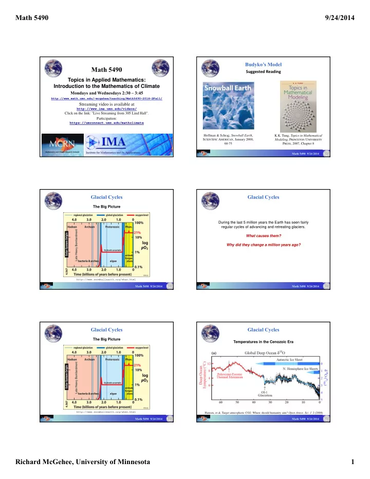
Topics in Applied Mathematics: Introduction to the Mathematics of Climate

Mondays and Wednesdays 2:30 – 3:45

http://www.math.umn.edu/~mcgehee/teaching/Math5490-2014-2Fall/

Streaming video is available at

http://www.ima.umn.edu/videos/

Click on the link: "Live Streaming from 305 Lind Hall". Participation:

https://umconnect.umn.edu/mathclimate

Math 5490

Budyko’s Model

Suggested Reading

Math 5490 9/24/2014

Hoffman & Schrag, Snowball Earth, SCIENTIFIC AMERICAN, January 2000, 68-75 K.K. Tung, Topics in Mathematical Modeling, PRINCETON UNIVERSITY PRESS, 2007, Chapter 8

Glacial Cycles

http://www.snowballearth.org/when.html

The Big Picture

Math 5490 9/24/2014

Glacial Cycles

During the last 5 million years the Earth has seen fairly regular cycles of advancing and retreating glaciers. What causes them? Why did they change a million years ago?

Math 5490 9/24/2014

Glacial Cycles

http://www.snowballearth.org/when.html

The Big Picture

Math 5490 9/24/2014

Glacial Cycles

Hansen, et al, Target atmospheric CO2: Where should humanity aim? Open Atmos. Sci. J. 2 (2008)

Temperatures in the Cenozoic Era

Math 5490 9/24/2014

SLIDE 2

Math 5490 9/24/2014 Richard McGehee, University of Minnesota 2

18O as a Climate Proxy

Foraminifera absorb more 18O into their skeletons when the water temperature is lower and when more 18O is in the water. Thus higher concentrations of 18O in foraminifera fossils indicate lower ocean temperatures and higher glacier volume. The isotope 16O preferentially evaporates from the ocean and is sequestered in glaciers, leaving the heavier isotope 18O more highly concentrated in the ocean. Thus

• ceanic concentration of the isotope

18O is higher during glacial periods.

Glacial Cycles

Math 5490 9/24/2014

18O in Foraminifera Fossils During the Past 4.5 Myr

Lisiecki, L. E., and M. E. Raymo (2005), A Pliocene-Pleistocene stack of 57 globally distributed benthic d18O records, Paleoceanography,20, PA1003, doi:10.1029/2004PA001071.

2.5 3 3.5 4 4.5 5 5.5 ‐4500 ‐4000 ‐3500 ‐3000 ‐2500 ‐2000 ‐1500 ‐1000 ‐500 Benthic Data (δ18O) time (Kyr)

Glacial Cycles

Math 5490 9/24/2014

2.5 3 3.5 4 4.5 5 5.5 ‐1000 ‐900 ‐800 ‐700 ‐600 ‐500 ‐400 ‐300 ‐200 ‐100 Benthic Data (δ18O) time (Kyr)

18O in Foraminifera Fossils During the Past 1.0 Myr

Glacial Cycles

Lisiecki, L. E., and M. E. Raymo (2005), A Pliocene-Pleistocene stack of 57 globally distributed benthic d18O records, Paleoceanography,20, PA1003, doi:10.1029/2004PA001071. Math 5490 9/24/2014

Recent (last 400 Kyr) Temperature Cycles Vostok Ice Core Data

J.R. Petit, et al (1999) Climate and atmospheric history of the past 420,000 years from the Vostok ice core, Antarctica, Nature 399, 429-436.

Glacial Cycles

Math 5490 9/24/2014

What Causes Glacial Cycles?

The glacial cycles are driven by the variations in the Earth’s orbit (Milankovitch Cycles), causing a variation in incoming solar radiation (insolation). This hypothesis is widely accepted, but also widely regarded as insufficient to explain the observations. The additional hypothesis is that there are feedback mechanisms and/or triggering mechanisms that amplify the Milankovitch cycles. What these feedbacks are and how they work are not fully understood. Widely Accepted Hypothesis

Glacial Cycles

Math 5490 9/24/2014

Heat Balance Historical Overview of Climate Change Science, IPCC AR4, p.96

http://ipcc-wg1.ucar.edu/wg1/Report/AR4WG1_Print_CH01.pdf

Glacial Cycles

Math 5490 9/24/2014

SLIDE 3

Math 5490 9/24/2014 Richard McGehee, University of Minnesota 3

Earth’s Orbit Kepler’s First Law: The orbit of every planet is an ellipse with the Sun at one of the two foci.

Eccentricity = c/a

Johannes Kepler (1571-1630)

Glacial Cycles

Math 5490 9/24/2014

Eccentricity

John Imbrie & Katherine Palmer Imbrie, Ice Ages: Solving the Mystery, Harvard Univ. Press, 1979.

Glacial Cycles

Math 5490 9/24/2014

Eccentricity Perihelion: 91.5x106 mi Aphelion: 94.5x106 mi Semimajor axis: 93x106 mi Eccentricity: 1.5/93 = 0.016

Glacial Cycles

Math 5490 9/24/2014

Eccentricity Perihelion: 91.5 Aphelion: 94.5 Change in radius: 3/93 = 3.2% Change in insolation: 6.4% Six percent less insolation in the southern winter than the northern winter. 6.4% of 342 W/m2 = 22 W/m2

Glacial Cycles

Math 5490 9/24/2014

Solar intensity at distance r from the sun:

2 2

m

E

r 

   

2 2 2 2

Joules 4 4

P P E E

Kr Kr dt dt r t r t        Total annual solar input (P = one year (in seconds)): Solar output:

26

4 10 Watts K   Cross section of Earth:

   

2 2 Wm

4 K Q t r t 



 Global solar input:

 

2 2 W

4

E

Kr r t

Glacial Cycles

Global Annual Average Insolation

Math 5490 9/24/2014

Specific angular momentum (angular momentum per unit mass):

2 2 1

m s r 



   Mean annual solar input: Total annual solar input:

 

2 2 2 2 2 2

Joules 4 4 4 2

P P E E E E

Kr Kr Kr Kr dt dt d r t



              





2

Watts 2

E

Kr P   Mean annual solar intensity on the Earth’s surface:

2 2 2

1 = W m 2 4 8

E E

Kr K P r P  



  

Glacial Cycles

Global Annual Average Insolation

Math 5490 9/24/2014

SLIDE 4

Math 5490 9/24/2014 Richard McGehee, University of Minnesota 4

Kepler’s Third Law:

3 2

P a  a = semimajor axis Derived from Kepler:

2 2

1 e a    e = eccentricity Global Annual Average Insolation Mean annual solar intensity:

3 2 1 2 2 2 2 2

ˆ ˆ = = Wm 8 1 1 K Ka a Ka P e e



  

Glacial Cycles

Math 5490 9/24/2014

Planetary Motion

 

2 3 2 1 n i j j i i i j j i j i

Gm m x x d x m dt x x

 

  



The orbits of all the planets can be computed (both forward and backward in time) for billions of years.

Isaac Newton 1642-1727 Jacques Laskar (1955-)

Glacial Cycles

Math 5490 9/24/2014

2 2

ˆ 1 Ka e  Laskar: Semi major axis does not change much: 0.005% corresponding to .01% change in global average insolation

• J. Laskar, et al (2004) A long-term numerical solution for the insolation quantities of the Earth, Astronomy &

Astrophysics 428, 261–285.

Glacial Cycles

Global Annual Average Insolation

Math 5490 9/24/2014

• J. Laskar, et al (2004) A long-term numerical solution for the insolation quantities of the Earth, Astronomy &

Astrophysics 428, 261–285.

The effect due to eccentricity is more significant, but not that much: As e varies between 0 and 0.06, (1-e2)-1/2 varies between 1 and 1.0018, or about 0.2%. (Twenty times the effect due to a.)

Eccentricity

Note periods of about 100 kyr and 400 kyr.

0.00 0.01 0.02 0.03 0.04 0.05 0.06 ‐1000 ‐900 ‐800 ‐700 ‐600 ‐500 ‐400 ‐300 ‐200 ‐100 eccentricity time (Kyr)

Glacial Cycles

Math 5490 9/24/2014

Obliquity

http://upload.wikimedia.org/wikipedia/commons/6/61/AxialTiltObliquity.png

Glacial Cycles

Math 5490 9/24/2014

Note period of about 41 Kyr.

22.0 22.5 23.0 23.5 24.0 24.5 ‐1000 ‐900 ‐800 ‐700 ‐600 ‐500 ‐400 ‐300 ‐200 ‐100

• bliquity (degrees)

time (Kyr)

Glacial Cycles

Obliquity

• J. Laskar, et al (2004) A long-term numerical solution for the insolation quantities of the Earth, Astronomy &

Astrophysics 428, 261–285. Math 5490 9/24/2014

SLIDE 5

Math 5490 9/24/2014 Richard McGehee, University of Minnesota 5

Precession

http://earthobservatory.nasa.gov/Library/Giants/Milankovitch/milankovitch_2.html

Glacial Cycles

Math 5490 9/24/2014

Precession Index

Note period of about 23 Kyr. index = e sinρ, where e = eccentricity and ρ = precession angle (measured from spring equinox)

‐0.06 ‐0.04 ‐0.02 0.00 0.02 0.04 0.06 ‐1000 ‐900 ‐800 ‐700 ‐600 ‐500 ‐400 ‐300 ‐200 ‐100 time (Kyr)

Glacial Cycles

• J. Laskar, et al (2004) A long-term numerical solution for the insolation quantities of the Earth, Astronomy &

Astrophysics 428, 261–285. Math 5490 9/24/2014 http://en.wikipedia.org/wiki/Milankovitch_cycles

Glacial Cycles

Math 5490 9/24/2014

Eccentricity

John Imbrie & Katherine Palmer Imbrie, Ice Ages: Solving the Mystery, Harvard Univ. Press, 1979.

Glacial Cycles

Math 5490 9/24/2014

Daily Average Insolation at Summer Solstice at 65° N          

2

, , , , , cos cos cos cos sin sin sin sin cos 4 K I r r                  



          

Insolation at a point on the Earth’s surface (φ,γ) = (latitude, longitude) (r,θ) = position of Earth in orbital plane β = obliquity angle ρ = precession angle    

   

2 2 2 2

1 sin 1 , , , cos cos cos sin sin 2 1 e I e Q d e



          



     



Daily average insolation at latitude φ at summer solstice

Glacial Cycles

Math 5490 9/24/2014

Daily Average Insolation at Summer Solstice at 65° N

420 440 460 480 500 520 540 560 580 ‐1000 ‐900 ‐800 ‐700 ‐600 ‐500 ‐400 ‐300 ‐200 ‐100 W/m^2 Kyr

Glacial Cycles

Math 5490 9/24/2014

SLIDE 6

Math 5490 9/24/2014 Richard McGehee, University of Minnesota 6

http://en.wikipedia.org/wiki/Milankovitch_cycles

Glacial Cycles

Math 5490 9/24/2014 Milutin Milankovitch 1879-1958

Milutin Milankovitch was a Serbian mathematician and professor at the University of Belgrade. In 1920 he published his seminal work on the relation between insolation and the Earth’s orbital parameters. In 1941 he published a book explaining his entire theory. His work was not fully accepted until 1976. Who was Milankovitch?

Glacial Cycles

Math 5490 9/24/2014

What happened in 1976? Hays, Imbrie, and Shackleton, “Variations in the Earth's Orbit: Pacemaker of the Ice Ages,” Science 194, 10 December 1976. “It is concluded that changes in the earth's

• rbital geometry are the fundamental cause
• f the succession of Quaternary ice ages.”

James D. Hays John Imbrie Nicholas Shackleton

Glacial Cycles

Math 5490 9/24/2014

Solar Forcing (Hays, et al) Hays, et al, Science 194 (1976), p. 1125

Glacial Cycles

Math 5490 9/24/2014

1) Three indices of global climate have been monitored in the record of the past 450,000 years in Southern Hemisphere

• cean-floor sediments.

2) ... climatic variance of these records is concentrated in three discrete spectral peaks at periods of 23,000, 42,000, and approximately 100,000 years. These peaks correspond to the dominant periods of the earth's solar orbit, and contain respectively about 10, 25, and 50 percent of the climatic variance. Hays, et al, Summary

Glacial Cycles

Hays, et al, Science 194 (1976), p. 1125

Math 5490 9/24/2014

3) The 42,000-year climatic component has the same period as variations in the obliquity of the earth's axis and retains a constant phase relationship with it. 4) The 23,000-year portion of the variance displays the same periods (about 23,000 and 19,000 years) as the quasiperiodic precession index. 5) The dominant, 100,000-year climatic component has an average period close to, and is in phase with, orbital eccentricity. Unlike the correlations between climate and the higher-frequency orbital variations (which can be explained on the assumption that the climate system responds linearly to orbital forcing), an explanation of the correlation between climate and eccentricity probably requires an assumption of nonlinearity.

Glacial Cycles

Hays, et al, Science 194 (1976), p. 1125

Hays, et al, Summary

Math 5490 9/24/2014

SLIDE 7

Math 5490 9/24/2014 Richard McGehee, University of Minnesota 7

6) It is concluded that changes in the earth's orbital geometry are the fundamental cause of the succession of Quaternary ice ages. 7) A model of future climate based on the observed orbital-climate relationships, but ignoring anthropogenic effects, predicts that the long-term trend over the next seven thousand years is toward extensive Northern Hemisphere glaciation*. *Quoted by George Will, Washington Post, February 5, 2009

Glacial Cycles

Hays, et al, Summary

Hays, et al, Science 194 (1976), p. 1125

Math 5490 9/24/2014

The Coming Ice Age eccentricity

• bliquity

Antarctic temperature record

Glacial Cycles

0.01 0.02 0.03 0.04 0.05 0.06 ‐450 ‐400 ‐350 ‐300 ‐250 ‐200 ‐150 ‐100 ‐50 50 100 eccentricity kyr 22 22.5 23 23.5 24 24.5 ‐450 ‐400 ‐350 ‐300 ‐250 ‐200 ‐150 ‐100 ‐50 50 100

• bliquity

kyr

• 10
• 8
• 6
• 4
• 2

2 4

• 450
• 400
• 350
• 300
• 250
• 200
• 150
• 100
• 50

δ°C kyr

Math 5490 9/24/2014

1800 1820 1840 1860 1880 1900 1920 1940 1960 1980 2000

Agassiz announces glacial theory

History of Discovery

Adhemar explains glacial cycles Humboldt debunks Adhemar Croll explains glacial cycles Evidence of multiple ice ages discovered in Illinois Magnetic reversals discovered Milankovitch explains glacial cycles

18O theory developed

climate fluctuations found in ocean cores paleomagnetic time scale developed Hays, et al

Glacial Cycles

Fourier Math 5490 9/24/2014

Suggested Reading

John Imbrie & Katherine Palmer Imbrie, Ice Ages: Solving the Mystery, HARVARD UNIVERSITY PRESS, 1979

Math 5490 9/24/2014

Glacial Cycles