Math 5490 10/1/2014 Glacial Cycles Math 5490 October 1, 2014 - - PDF document

math 5490 10 1 2014
SMART_READER_LITE
LIVE PREVIEW

Math 5490 10/1/2014 Glacial Cycles Math 5490 October 1, 2014 - - PDF document

Math 5490 10/1/2014 Glacial Cycles Math 5490 October 1, 2014 Topics in Applied Mathematics: Who was Milankovitch? Introduction to the Mathematics of Climate Mondays and Wednesdays 2:30 3:45 Milutin Milankovitch was a Serbian


slide-1
SLIDE 1

Math 5490 10/1/2014 Richard McGehee, University of Minnesota 1

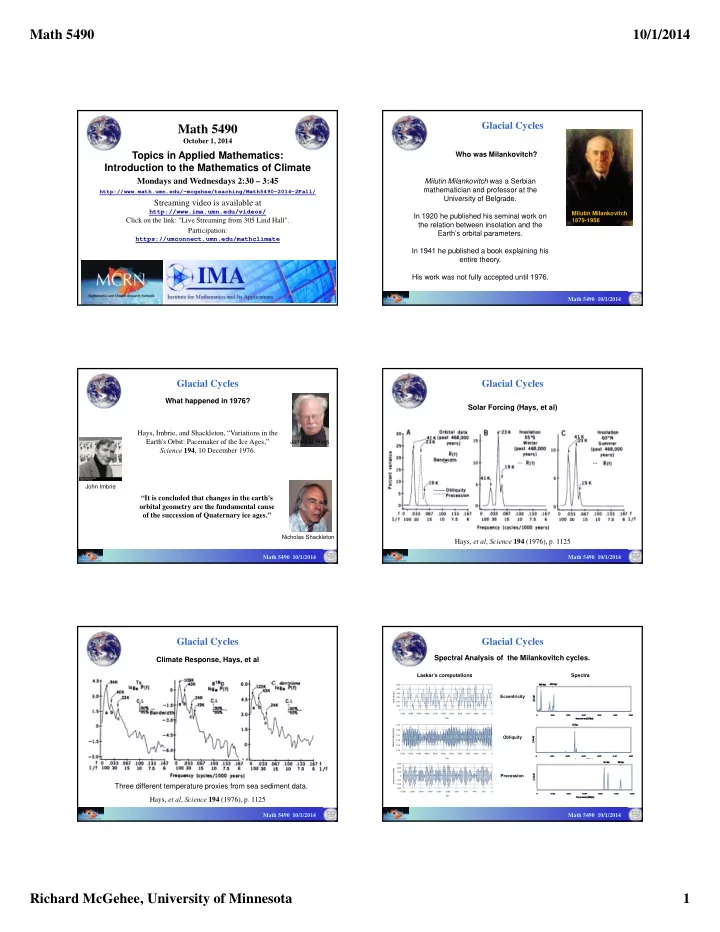
Topics in Applied Mathematics: Introduction to the Mathematics of Climate

Mondays and Wednesdays 2:30 – 3:45

http://www.math.umn.edu/~mcgehee/teaching/Math5490-2014-2Fall/

Streaming video is available at

http://www.ima.umn.edu/videos/

Click on the link: "Live Streaming from 305 Lind Hall". Participation:

https://umconnect.umn.edu/mathclimate

Math 5490

October 1, 2014

Milutin Milankovitch 1879-1958

Milutin Milankovitch was a Serbian mathematician and professor at the University of Belgrade. In 1920 he published his seminal work on the relation between insolation and the Earth’s orbital parameters. In 1941 he published a book explaining his entire theory. His work was not fully accepted until 1976. Who was Milankovitch?

Glacial Cycles

Math 5490 10/1/2014

What happened in 1976? Hays, Imbrie, and Shackleton, “Variations in the Earth's Orbit: Pacemaker of the Ice Ages,” Science 194, 10 December 1976. “It is concluded that changes in the earth's

  • rbital geometry are the fundamental cause
  • f the succession of Quaternary ice ages.”

James D. Hays John Imbrie Nicholas Shackleton

Glacial Cycles

Math 5490 10/1/2014

Solar Forcing (Hays, et al) Hays, et al, Science 194 (1976), p. 1125

Glacial Cycles

Math 5490 10/1/2014

Climate Response, Hays, et al Three different temperature proxies from sea sediment data.

Glacial Cycles

Hays, et al, Science 194 (1976), p. 1125

Math 5490 10/1/2014

Spectral Analysis of the Milankovitch cycles.

0.01 0.02 0.03 0.04 0.05 0.06 ‐5500 ‐5000 ‐4500 ‐4000 ‐3500 ‐3000 ‐2500 ‐2000 ‐1500 ‐1000 ‐500 eccentricity Kyr 22.0 22.5 23.0 23.5 24.0 24.5 ‐5500 ‐5000 ‐4500 ‐4000 ‐3500 ‐3000 ‐2500 ‐2000 ‐1500 ‐1000 ‐500

  • bliquity (degrees)

Kyr ‐0.06 ‐0.04 ‐0.02 0.02 0.04 0.06 ‐2000 ‐1800 ‐1600 ‐1400 ‐1200 ‐1000 ‐800 ‐600 ‐400 ‐200 precession index Kyr

Laskar’s computations Spectra

Eccentricity Obliquity Precession

Glacial Cycles

Math 5490 10/1/2014

slide-2
SLIDE 2

Math 5490 10/1/2014 Richard McGehee, University of Minnesota 2

Summer Solstice 65°N

Glacial Cycles

420 460 500 540 580 ‐5500 ‐5000 ‐4500 ‐4000 ‐3500 ‐3000 ‐2500 ‐2000 ‐1500 ‐1000 ‐500 W/m2 Kyr

eccentricity?

  • bliquity

precession

Math 5490 10/1/2014

Milankovitch vs. Climate

Glacial Cycles

eccentricity?

  • bliquity

precession

Math 5490 10/1/2014

Hays, et al, Science 194 (1976), p. 1127 Hays, et al, Summary Increasing contribution Forcing precession

  • bliquity

eccentricity eccentricity

  • bliquity

precession Response Hays’ explanation is that there are nonlinear feedbacks. Are there other explanations?

Glacial Cycles

Math 5490 10/1/2014

Climate Response (Zachos, et al) Zachos, et al, Science 292 (2001), p. 689 Power spectrum of climate for the last 4.5

  • Myr. Note the peaks

at 41Kyr and 100 Kyr.

Glacial Cycles

Math 5490 10/1/2014

Zachos, et al, Summary Increasing contribution Nonlinear effects? Other explanations? Zachos, et al, Science 292 (2001), p. 689 Forcing precession

  • bliquity

eccentricity

  • bliquity

eccentricity precession Response

Glacial Cycles

Math 5490 10/1/2014

0.00 0.01 0.02 0.03 0.04 0.05 0.06 power frequency (1/Kyr) 100 Kyr 41 Kyr 23 Kyr

precession

  • bliquity

eccentricity

Spectral Analysis of the Climate Data

2.5 3.0 3.5 4.0 4.5 5.0 5.5 ‐5500 ‐5000 ‐4500 ‐4000 ‐3500 ‐3000 ‐2500 ‐2000 ‐1500 ‐1000 ‐500 δ18O Kyr

Glacial Cycles

Math 5490 10/1/2014

slide-3
SLIDE 3

Math 5490 10/1/2014 Richard McGehee, University of Minnesota 3

0.00 0.01 0.02 0.03 0.04 0.05 0.06 power frequency (1/Kyr) 100 Kyr 41 Kyr 23 Kyr

precession

  • bliquity

eccentricity

Spectral Analysis of the Climate Data

2.5 3.0 3.5 4.0 4.5 5.0 5.5 ‐5500 ‐5000 ‐4500 ‐4000 ‐3500 ‐3000 ‐2500 ‐2000 ‐1500 ‐1000 ‐500 δ18O Kyr

Conclusion Remains: The Milankovitch cycles “pace” the Earth’s climate. Exactly how is not so clear.

Glacial Cycles

Math 5490 10/1/2014

Increasing contribution If we assume that glaciation depends on annual average insolation instead of insolation at summer solstice, then forcing and response are aligned. Forcing

  • bliquity

eccentricity

  • bliquity

eccentricity Response precession precession

Glacial Cycles

Zachos Summary (Revised)

Math 5490 10/1/2014

Something’s Missing

Glacial Cycles

22.0 22.5 23.0 23.5 24.0 24.5 ‐5500 ‐5000 ‐4500 ‐4000 ‐3500 ‐3000 ‐2500 ‐2000 ‐1500 ‐1000 ‐500

  • bliquity (degrees)

Kyr

2.5 3 3.5 4 4.5 5 5.5 ‐6000 ‐5000 ‐4000 ‐3000 ‐2000 ‐1000 d18O Kyr

Lisiecki‐Raymo Stack

  • bliquity

climate

Math 5490 10/1/2014 data power spectrum

Glacial Cycles

2.5 3 3.5 4 4.5 5 5.5 ‐6000 ‐5000 ‐4000 ‐3000 ‐2000 ‐1000 d18O Kyr

Lisiecki‐Raymo Stack 0.00 0.01 0.02 0.03 0.04 0.05 0.06 power frequency (1/Kyr) 100 Kyr 41 Kyr 23 Kyr

eccentricity?

  • bliquity

precession

Something’s Missing

Math 5490 10/1/2014 Last Million Years is Different

Glacial Cycles

  • 5 to -1 Myr

0.00 0.01 0.02 0.03 0.04 0.05 0.06 power frequency (1/Kyr) 100 Kyr 41 Kyr 23 Kyr

eccentricity?

  • bliquity

precession

  • 1 to 0 Myr
  • 5 to 0 Myr

A transition

  • ccurred about
  • ne million

years ago: the amplitude increased and the dominant period changed from 41 kyr to 100 kyr.

Math 5490 10/1/2014

What’s up with the Last Million Years?

Glacial Cycles

100,000 Year Problem: Why did the eccentricity signal become so dominant during the last million years? 400,000 Year Problem: If the last million years is dominated by eccentricity, what happened to the 400,000 year cycle?

eccentricity

0.00 0.01 0.02 0.03 0.04 0.05 0.06 power frequency (1/Kyr) 100 Kyr 41 Kyr 23 Kyr

eccentricity?

  • bliquity

precession

data

Math 5490 10/1/2014

slide-4
SLIDE 4

Math 5490 10/1/2014 Richard McGehee, University of Minnesota 4

Budyko’s Model

( )(1 ( , )) ( ) ( ) T R Qs y y A BT C T T t          

heat transport OLR albedo insolation heat capacity surface temperature sin(latitude)

1

( ) T T y dy   ice line reduces to

 

( ) ( )

c

d T T h dt       

Math 5490 10/1/2014

Glacial Cycles

Budyko’s Model

( ) d h dt   

stable equilibrium η*

‐10 ‐8 ‐6 ‐4 ‐2 2 4 6 0.1 0.2 0.3 0.4 0.5 0.6 0.7 0.8 0.9 1

h(η) η

Math 5490 10/1/2014

Glacial Cycles

Budyko’s Model

( ) d h dt    ( )(1 ( , )) ( ) ( ) T R Qs y y A BT C T T t          

The function h , and hence the equilibrium solution η*, depends on all the parameters of the Budyko model. In particular, η* depends on Q and s(y) , which depend on the eccentricity e and the obliquity β .  

2

1 Q Q e e  

 

 

2 2 2 2

2 , 1 1 sin cos cos s y y y d

             * *( , ) e    

Math 5490 10/1/2014

Glacial Cycles

McGehee & Lehman, A Paleoclimate Model of Ice-Albedo Feedback Forced by Variations in Earth’s Orbit, SIAM J. APPLIED DYNAMICAL SYSTEMS 11 (2012), 684–707.

Budyko’s Model

( , , ) d h e dt    

The eccentricity e and the obliquity β are given by Laskar as functions of time.

*( ) *( ( ), ( )) t e t t    

Math 5490 10/1/2014

Glacial Cycles

McGehee & Lehman, A Paleoclimate Model of Ice-Albedo Feedback Forced by Variations in Earth’s Orbit, SIAM J. APPLIED DYNAMICAL SYSTEMS 11 (2012), 684–707.

0.01 0.02 0.03 0.04 0.05 0.06 ‐5500 ‐5000 ‐4500 ‐4000 ‐3500 ‐3000 ‐2500 ‐2000 ‐1500 ‐1000 ‐500 eccentricity Kyr 22.0 22.5 23.0 23.5 24.0 24.5 ‐5500 ‐5000 ‐4500 ‐4000 ‐3500 ‐3000 ‐2500 ‐2000 ‐1500 ‐1000 ‐500

  • bliquity (degrees)

Kyr

Therefore, the stable equilibrium ice line is a function of time: Budyko’s Model

( , , ) d h e dt     stable equilibrium η*(e(t),β(t))

‐10 ‐8 ‐6 ‐4 ‐2 2 4 6 0.1 0.2 0.3 0.4 0.5 0.6 0.7 0.8 0.9 1

h(η) η

Math 5490 10/1/2014

Glacial Cycles

Budyko’s Model

0.91 0.92 0.93 0.94 ‐5500 ‐5000 ‐4500 ‐4000 ‐3500 ‐3000 ‐2500 ‐2000 ‐1500 ‐1000 ‐500 sin(latitude) Kyr

ice line GMT

Glacial Cycles

Math 5490 10/1/2014 McGehee & Lehman, SIAM J. APPLIED DYNAMICAL SYSTEMS 11 (2012), 684–707.

slide-5
SLIDE 5

Math 5490 10/1/2014 Richard McGehee, University of Minnesota 5

2.5 3 3.5 4 4.5 5 5.5 ‐6000 ‐5000 ‐4000 ‐3000 ‐2000 ‐1000 d18O Kyr Lisiecki‐Raymo Stack 0.91 0.92 0.93 0.94 ‐5500 ‐5000 ‐4500 ‐4000 ‐3500 ‐3000 ‐2500 ‐2000 ‐1500 ‐1000 ‐500

sin(latitude) Kyr

Glacial Cycles

Math 5490 10/1/2014

Budyko’s Model

2.5 3 3.5 4 4.5 5 5.5 ‐6000 ‐5000 ‐4000 ‐3000 ‐2000 ‐1000 d18O Kyr Lisiecki‐Raymo Stack 0.91 0.92 0.93 0.94 ‐5500 ‐5000 ‐4500 ‐4000 ‐3500 ‐3000 ‐2500 ‐2000 ‐1500 ‐1000 ‐500

sin(latitude) Kyr 0.00 0.01 0.02 0.03 0.04 0.05 0.06 power frequency (1/Kyr) 100 Kyr 41 Kyr 23 Kyr

eccentricity?

  • bliquity

precession

Glacial Cycles

Math 5490 10/1/2014

Budyko’s Model

Math 5490 10/1/2014

Glacial Cycles

McGehee & Lehman, SIAM J. APPLIED DYNAMICAL SYSTEMS 11 (2012), 684–707.

red: model simulation blue: data

Budyko’s Model

Math 5490 10/1/2014

Glacial Cycles

Budyko’s model of ice-albedo feedback produces a climate response driven primarily by obliquity cycles, consistent with the dominance of obliquity in the climate data. The model fails to produce: 1. the amplitude changes over the past 5 million years, and 2. the frequency change 1 million years ago (“mid-Pleistocene transition). Budyko’s Model

Math 5490 10/1/2014

Glacial Cycles

MATLAB Program: PaleoBudyko

Download from http://www.math.umn.edu/~mcgehee/Software/ Budyko’s Model

Math 5490 10/1/2014

Glacial Cycles

Some Recent Developments Modeling Glacial Cycles

slide-6
SLIDE 6

Math 5490 10/1/2014 Richard McGehee, University of Minnesota 6

Andrew McC. Hogg, "Glacial cycles and carbon dioxide: A conceptual model," Geophysical Research Letters 35 (2008).

Hogg’s Model

Glacial Cycles

       

4 1 max

, max ,0 . dT c S t G C T dt dC dT V W W C C C dt dt                  

CO2 outgassing weathering volcanos

   

2 sin ln

i i i

t S t S S C G C G A C                  

insolation greenhouse forcing

surface temperature atmospheric carbon

Math 5490 10/1/2014

Glacial Cycles

Hogg’s Model Hogg’s model shows how the carbon cycle can act as a feedback amplifying and modifying the insolation forcing, but the forcing is somewhat artificial, and the triggering mechanism is difficult to justify. What if the 100,000 year glacial cycle is not driven by eccentricity, but is a natural oscillation of the Earth’s climate? Saltzman and Maasch suggested just such a model.

Glacial Cycles

Hogg’s Model

Math 5490 10/1/2014

   

2 2

X X Y uM t Y pZ rY sZ Z Y Z q X Z               

global ice mass atmospheric CO2

  • cean circulation

Milankovitch forcing

Barry Salzman and Kirk A. Maasch, "A Low-Order Dynamical Model of Global Climatic Variability Over the Full Pleistocene," Journal of Geophysical Research 95 (D2), 1955-1963 (1990)

Glacial Cycles

Math 5490 10/1/2014

Salzman-Maasch Model

Glacial Cycles

Math 5490 10/1/2014

unforced

Salzman-Maasch Model

forced

Glacial Cycles

Salzman-Maasch Model

Math 5490 10/1/2014

slide-7
SLIDE 7

Math 5490 10/1/2014 Richard McGehee, University of Minnesota 7

The Salzman-Maasch model shows how the carbon cycle and the ocean currents can interact to produce unforced oscillations with periods of about 100,000 years. The same model with slightly different parameters can exhibit stationary behavior. By forcing the model with Milankovitch cycles and by slowly varying the parameters over the last two million years, they can produce a bifurcation from small oscillations tracking the Milankovitch cycles to large oscillations with a dominant 100,000 year period. Seems like a nice idea, but it is not widely accepted as the explanation, and it has some problems.

Glacial Cycles

Salzman-Maasch Model

Math 5490 10/1/2014

The Hopf bifurcation explanation seems to have two serious problems (“cosmic coincidences”). 1. Why does the intrinsic period of the glacial cycles just happen to have the same period as the eccentricity cycles? 2. Why does the phase of the glacial cycles agree with the phase of the obliquity and eccentricity cycles? Samantha Oestreicher, PhD Thesis, 2014.

Glacial Cycles

Salzman-Maasch Model

Math 5490 10/1/2014