Math 5490 10/6/2014 Glacial Cycles Math 5490 October 6, 2014 - - PDF document

Math 5490 10/6/2014 Richard McGehee, University of Minnesota 1

Topics in Applied Mathematics: Introduction to the Mathematics of Climate

Mondays and Wednesdays 2:30 – 3:45

http://www.math.umn.edu/~mcgehee/teaching/Math5490-2014-2Fall/

Streaming video is available at

http://www.ima.umn.edu/videos/

Click on the link: "Live Streaming from 305 Lind Hall". Participation:

https://umconnect.umn.edu/mathclimate

Math 5490

October 6, 2014

Math 5490 10/6/2014

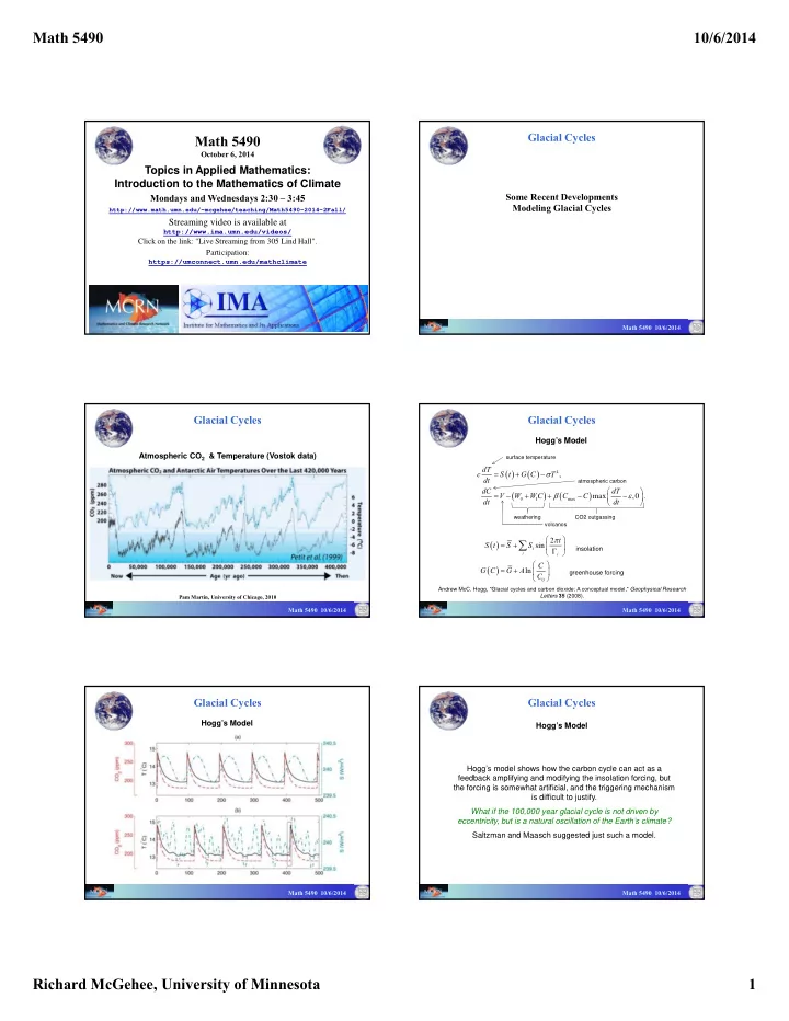
Glacial Cycles

Some Recent Developments Modeling Glacial Cycles

Pam Martin, University of Chicago, 2010

Atmospheric CO2 & Temperature (Vostok data)

Glacial Cycles

Math 5490 10/6/2014

Andrew McC. Hogg, "Glacial cycles and carbon dioxide: A conceptual model," Geophysical Research Letters 35 (2008).

Hogg’s Model

Glacial Cycles

       

4 1 max

, max ,0 . dT c S t G C T dt dC dT V W W C C C dt dt                  

CO2 outgassing weathering volcanos

   

2 sin ln

i i i

t S t S S C G C G A C                  



insolation greenhouse forcing

surface temperature atmospheric carbon

Math 5490 10/6/2014

Glacial Cycles

Hogg’s Model

Math 5490 10/6/2014

Hogg’s model shows how the carbon cycle can act as a feedback amplifying and modifying the insolation forcing, but the forcing is somewhat artificial, and the triggering mechanism is difficult to justify. What if the 100,000 year glacial cycle is not driven by eccentricity, but is a natural oscillation of the Earth’s climate? Saltzman and Maasch suggested just such a model.

Glacial Cycles

Hogg’s Model

Math 5490 10/6/2014

Math 5490 10/6/2014 Richard McGehee, University of Minnesota 2

   

2 2

X X Y uM t Y pZ rY sZ Z Y Z q X Z               

global ice mass atmospheric CO2

• cean circulation

Milankovitch forcing

Barry Salzman and Kirk A. Maasch, "A Low-Order Dynamical Model of Global Climatic Variability Over the Full Pleistocene," Journal of Geophysical Research 95 (D2), 1955-1963 (1990)

Glacial Cycles

Salzman-Maasch Model

Math 5490 10/6/2014

Glacial Cycles

unforced

Salzman-Maasch Model

Math 5490 10/6/2014

forced

Glacial Cycles

Salzman-Maasch Model

Math 5490 10/6/2014

The Salzman-Maasch model shows how the carbon cycle and the ocean currents can interact to produce unforced oscillations with periods of about 100,000 years. The same model with slightly different parameters can exhibit stationary behavior. By forcing the model with Milankovitch cycles and by slowly varying the parameters over the last two million years, they can produce a bifurcation from small oscillations tracking the Milankovitch cycles to large oscillations with a dominant 100,000 year period. Seems like a nice idea (especially by mathematicians, since it looks like a “Hopf Bifurcation”,) but it is not widely accepted as the explanation, and it has some problems.

Glacial Cycles

Salzman-Maasch Model

Math 5490 10/6/2014

The bifurcation explanation seems to have two serious problems (“cosmic coincidences”). 1. Why does the intrinsic period of the glacial cycles just happen to have the same period as the eccentricity cycles? 2. Why does the phase of the glacial cycles agree with the phase of the obliquity and eccentricity cycles? Samantha Oestreicher, PhD Thesis, 2014.

Glacial Cycles

Salzman-Maasch Model

Math 5490 10/6/2014

Huybers’ Analysis of Deglaciations

Peter Huybers, "Glacial variability over the last two million years: an extended depth-derived age model, continuous

• bliquity pacing, and the Pleistocene progression," Quaternary Science Reviews 26, 37-55 (2007).

Glacial Cycles

Math 5490 10/6/2014

Issue of Circular Reasoning Data sets (stacks of data from individual sediment cores) are usually “orbitally tuned”, i.e., the “age model” is adjusted so the cycles in the data line up with Milankovitch cycles. Using tuned data sets to conclude that Milankovitch theory is valid is circular reasoning. Huybers rederived the “age model” for a Pleistocene data set without using orbital tuning. He concluded that the deglaciations are triggered by obliquity.

Math 5490 10/6/2014 Richard McGehee, University of Minnesota 3

Huybers’ Analysis of Deglaciations

Red dots: deglaciations.

Glacial Cycles

Math 5490 10/6/2014

What are the horizontal red bars?

18O data are usually “orbitally tuned,” i.e., the age model is partially

determined by Milankovitch cycles. Huybers reworked the data using only geomagnetic markers, 18O events, and depth. Vertical black lines: Geomagnetic events Red dots: 18O events Yellow bars: Obliquity cycle skipped

Glacial Cycles

Huybers’ Analysis

Math 5490 10/6/2014

The ages for geomagnetic events are uncertain. Consequently, the

18O events are uncertain, and the entire age model is uncertain.

Glacial Cycles

Huybers’ Analysis

Math 5490 10/6/2014

Huyber’s age model agrees well with other age models, but contains no bias introduced by “orbital tuning”. Black: Huyber stack Red: Lisiecki and Raymo stack

Glacial Cycles

Huybers’ Analysis

Math 5490 10/6/2014

1

if if

t t t t t t t t

V V T V V T T at b c  

 

          : ice volume at time : threshold variable : rate of increase of ice volume : normalized obliquity

t t t

V t T   Units and constants t : Kyr V : chosen so that η = 1. θ’: mean zero and variance one a = 0.05 b = 126 c = 20

Glacial Cycles

Huybers’ Model of Deglaciations

Math 5490 10/6/2014

Glacial Cycles

Huybers’ Model

Math 5490 10/6/2014

Math 5490 10/6/2014 Richard McGehee, University of Minnesota 4

Huybers’ model produces the decline in temperature and the increase in period and amplitude of the glacial cycles, but it depends heavily on an unspecified decline in the sensitivity of the triggering mechanism over last two million years. Revised in 2011.

Glacial Cycles

Huybers’ Model

Math 5490 10/6/2014

The deglaciations are triggered by the following forcing function.

Glacial Cycles

1 2 1 2

sin( ) (1 )

t t t t

F e          eccentricity precession angle

• bliquity

t t t

e      and are parameters.   where Huybers’ 2011 Analysis of Deglaciations

Math 5490 10/6/2014

1

if if 110 25

t t t t t t t t

V V T V V T T F 

 

        : ice volume at time : threshold variable : rate of increase of ice volume

t t

V t T 

Glacial Cycles

1 2 1 2

sin( ) (1 )

t t t t

F e          Huybers’ 2011 Analysis of Deglaciations

Math 5490 10/6/2014 Peter Huybers, Combined obliquity and precession pacing of late Pleistocene deglaciations, NATURE 480 (2011), 229-232

Glacial Cycles

black = climate data grey = Ft red = simulation Huybers’ 2011 Model

Math 5490 10/6/2014

Glacial Cycles

Abe-Ouchi et al Ice Sheet Model Ayako Abe-Ouchi, Fuyuki Saito, Kenji Kawamura, Maureen E. Raymo, Jun’ichi Okuno, Kunio Takahashi & Heinz Blatter, “Insolation-driven 100,000-year glacial cycles and hysteresis of ice- sheet volume,” Nature 500 (2013), 190-193. doi:10.1038/nature12374 The larger the ice sheet, the more unstable it becomes, and the more sensitive it is to insolation. Once it begins to retreat, feedbacks cause a rapid pace. Animation available on Nature Web site:

http://www.nature.com/nature/journal/v500/n7461/full/nature12374.html#videos

Math 5490 10/6/2014

Questions

• 1. Did eccentricity play any role during the last million years?

Is the apparent 100 kyr cycle an artifact (Huybers)? Is it an intrinsic cycle in the climate system that coincidentally has a period of 100,000 years (Maasch and Saltzman)?

• 2. Is the CO2 feedback sufficient to explain the increasing amplitude

and period of the glacial cycles during the last million years, i.e., is it the mechanism behind the Huybers model.

• 3. Where does the atmospheric CO2 go during the glacial maxima?

The ocean? The land?

• 4. What will be the effect of the anthropogenic CO2?

Glacial Cycles

Math 5490 10/6/2014

Math 5490 10/6/2014 Richard McGehee, University of Minnesota 5

Pam Martin, University of Chicago, 2010

Atmospheric CO2 & Temperature (Vostok data)

Glacial Cycles

Math 5490 10/6/2014

‐10 ‐8 ‐6 ‐4 ‐2 2 4 6 8 10 12 150 200 250 300 350 400 450 δT (°C) CO2 (ppm)

Current conditions are well

• utside the

range recorded in the ice core data. Vostok Data

Glacial Cycles

Math 5490 10/6/2014

Vostok Data

‐10 ‐8 ‐6 ‐4 ‐2 2 4 6 8 10 12 150 200 250 300 350 400 450 δT (°C) CO2 (ppm)

Extrapolate linear regression to 400 ppm CO2.

Glacial Cycles

Math 5490 10/6/2014

Isotopes as Climate Proxies

How do we know the past climates?

Math 5490 10/6/2014

Isotopes as Proxies

What is this? δ18O (‰)

Hansen, et al, Target atmospheric CO2: Where should humanity aim? Open Atmos. Sci. J. 2 (2008) Math 5490 10/6/2014

http://eo.ucar.edu/staff/rrussell/climate/paleoclimate/sediment_proxy_records.html

Ocean Sediment Cores

Isotopes as Proxies

Math 5490 10/6/2014

Math 5490 10/6/2014 Richard McGehee, University of Minnesota 6

18O as a Climate Proxy

Foraminifera absorb more 18O into their skeletons when the water temperature is lower and when more 18O is in the water. Thus higher concentrations of 18O in foraminifera fossils indicate lower ocean temperatures and higher glacier volume. The isotope 16O preferentially evaporates from the ocean and is sequestered in glaciers, leaving the heavier isotope 18O more highly concentrated in the ocean. Thus

• ceanic concentration of the isotope

18O is higher during glacial periods.

Math 5490 9/24/2014

Isotopes as Proxies Isotopes as Proxies

What is this? δ18O (‰)

Hansen, et al, Target atmospheric CO2: Where should humanity aim? Open Atmos. Sci. J. 2 (2008) Math 5490 10/6/2014

What is this? δ18O (‰)

‰ : “per mil,” “per thousand” 1000‰ = 100% = 1 10‰ = 1% = 0.01 1‰ = 0.1% = 0.001

18O: Oxygen 18: 8 protons 8 electrons 10 neutrons 17O: Oxygen 17: 8 protons 8 electrons 9 neutrons 16O: Oxygen 16: 8 protons 8 electrons 8 neutrons

Most of the oxygen atoms on Earth are 16O. About 1 in 500 atoms is 18O. About 1 in 2500 is 17O. There are other oxygen isotopes, but they are unstable.

Isotopes as Proxies

Math 5490 10/6/2014