SLIDE 1
1
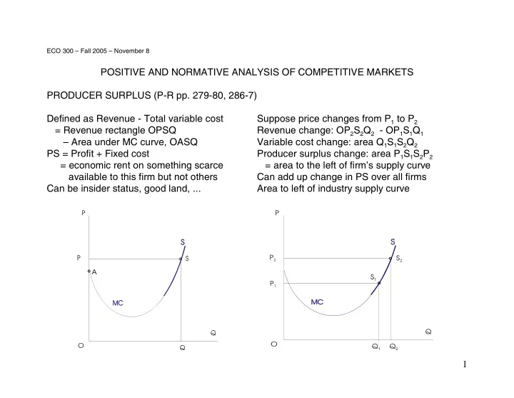
ECO 300 – Fall 2005 – November 8
POSITIVE AND NORMATIVE ANALYSIS OF COMPETITIVE MARKETS PRODUCER SURPLUS (P-R pp. 279-80, 286-7) Defined as Revenue - Total variable cost Suppose price changes from P1 to P2 = Revenue rectangle OPSQ Revenue change: OP2S2Q2 - OP1S1Q1 – Area under MC curve, OASQ Variable cost change: area Q1S1S2Q2 PS = Profit + Fixed cost Producer surplus change: area P1S1S2P2 = economic rent on something scarce = area to the left of firm’s supply curve available to this firm but not others Can add up change in PS over all firms Can be insider status, good land, ... Area to left of industry supply curve
SLIDE 2 2 OPTIMAL OUTPUT AND DEAD-WEIGHT LOSSES Consumer and producer surpluses are dollar measures of the benefit the two parties
- btain from engaging in the production and consumption of the good/service in question
There may be other benefits / costs, for example government revenues / disbursements Schematic exposition: Write net benefit from producing quantity Q as B(Q) – C(Q) First-order condition for maximization: B’(Q) - C’(Q) = 0
- r marginal benefit = marginal cost
But marginal benefit = consumers’ maximum willingness to pay for marginal unit of the good = height of demand curve at Q and marginal cost = height of supply curve at Q Therefore optimum is where the demand and supply curves intersect In figure, this is at E, quantity QE When Q1 < QE , MB1 > MC1 forgone net benefit = deadweight triangle E MB1 MC1 , output should be expanded When Q2 > QE , MB2 < MC2 forgone net benefit = deadweight triangle E MB2 MC2 , output should be contracted
SLIDE 3
3 Effect of a tax or a subsidy (P-R pp. 326-332) Tax: Quantity reduced from QE to QT Subsidy: Quantity increased from QE to QS Consumers pay CT - PE more per unit; Consumers pay PE - CS less per unit; Consumer surplus down by CTDTEPE Consumer surplus up by CSDSEPE Firms receive PE - FT less per unit; Firms receive FS - PE more per unit; Producer surplus down by FTSTEPE Producer surplus up by FSSSEPE CT - FT = amount of tax per unit of good FS - CS = amount of subsidy per unit of good Government revenue rectangle CTDTSTFT Government pays out rectangle CSDSSSFS Dead-weight loss: triangle EDTST Dead-weight loss: triangle EDSSS Tax and subsidy both create dead-weight losses - (competitive) equilibrium E is most efficient Other reasons may explain or justify tax / subsidy policies - [1] financing public good provision, [2] redistribution, [3] increase / decrease quantity of goods with + / – externalities, [4] political considerations: benefits to organized pivotal special interests, contributors etc.
SLIDE 4 4 APPLICATION – EU’S COMMON AGRICULTURAL POLICY (related to P-R pp. 314-6) Note - numbers are schematic; actual depend on commodity, year, special rates used for exchange ... Under free trade: P = 60 EU cons. = 120, prod. = 40 With price support at 130 EU cons. = 85, prod. = 145 Surplus 145 - 85 = 60 is sold on world market (or given away) (with reimports prohibited) EU consumer surplus loss = ½ (85+120) * (130-60) = 7175 EU producer surplus gain = ½ (145+40) * (130-60) = 6475 Note conflicting interests, typical in most international trade policy issues EU government revenue loss = (145-85) * (130-60) = 4200 Total EU loss = 7175 - 6475 + 4200 = 4900 This can be seen as the sum of two dead-weight loss triangles: ½ (120-85)(130-60) + ½ (145-40)(130-60) = ½ 35 * 70 + ½ 105 * 70 = ½ 140 * 70 In politics, concentrated and organized special interests can win, even if aggregate loss In reality, ROW supply curve is not perfectly elastic. The EU’s dumping of its surplus
- n the world market lowers the world price and inflicts further loss of ROW surplus,
usually harming producers in less-developed countries.
SLIDE 5
5 APPLICATION – US PETROLEUM SELF-SUFFICIENCY? (Related to P-R pp. 321-6) Quantities in millions of barrels per day, prices in dollars per barrel Approximate data for 2003: Price = 30, World production = consumption = 80, US consumption = 20, US production = 9, US import = Rest-of-world (ROW) export = 11 Assumptions: All supply and demand curves straight lines, with point elasticities at the data point US demand elasticity = 0.3 (rough estimate for medium-run adjustment) US supply elasticity = 1 (probably too high) Elasticity of ROW export supply to the US . 3 (exactly 30/11) (probably far too low) These imply equations for: US demand Q = 26 - 0.2 P . US inverse demand P = 130 - 5 Q US supply Q = 0.3 P , its inverse P = 3.33 Q US import demand Q = 26 - 0.5 P , its inverse P = 52 - 2 Q ROW’s supply to the US Q = P - 19, its inverse P = Q + 19 In isolation (“autarky”), US price would be 52, quantity 15.6 In free trade, P = 30, US consumption = 20, US production = 9, imports = 11
SLIDE 6
6 Now suppose the US imposes an import tariff (tax) of $15 per barrel Equilibrium: US imports = ROW exports = Q must be such that Price in the US = Price in ROW + 15, or 52 - 2 Q = Q + 19 + 15 3 Q = 18, or Q = 6 : US “dependence on foreign oil” has been cut nearly by half Price in US = 40, price in ROW = 25. US consumption = 18, US production = 12 US consumer surplus loss = ½ (18+20) * (40-30) = 190 (million dollars / day) US producer surplus gain = ½ (12+9) * (40-30) = 105 (So guess which interest group advocates and supports “energy independence” ! ) US government’s revenue from tariff = (40-25) * 6 = 90. So US net gain = 105 + 90 - 190 = 5 ROW loss = ½ (11+6) * (30 - 25) = 42.5 World-wide net loss = 42.5 - 5 = 37.5, equals dead-weight loss triangle ½ (40-25) * (11-6) Reason for gain : reduction in our purchase lowers the price at which ROW receives (Our consumers pay more, but our own government gets the difference) So the tariff is helping the US exercise “monopsony power” in world trade. To see this, redo the problem when ROW supply curve is flat at P = 30; then US loses