Run-Time Analysis of repeat Pr[ nobody disturbs ] 1 3 2 c := - PowerPoint PPT Presentation

Probabilistic Program Run-Time Analysis of repeat Pr[ nobody disturbs ] ≥ � 1 � 3 2 c := coin flip (0 . 5) Probabilistic Programs until ( c = heads ) Average Runtime Joost-Pieter Katoen 
 joint work with: Benjamin Kaminski, Christoph Matheja, and Federico Olmedo IFIP WG2.2 Meeting Singapore, September 2016

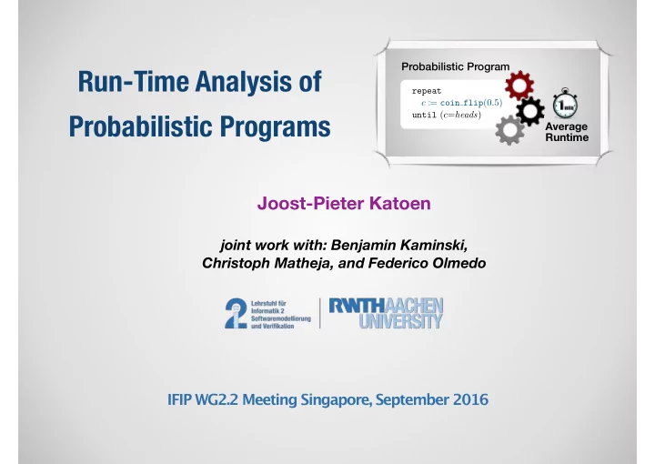
Probabilistic Programs — Basics What is a probabilistic program? imperative In this work “Ordinary” functional Program logical … + randomly choose a process with which communicate Probabilistic select a random prime in interval [1, n 2 ] Choice flip a (fair/biased) coin; Program behaviour ( input-output relation + runtime ) is determined by the outcome of its probabilistic choices. Program output is a probability distribution: v 1 with probability p 1 , v 2 with probability p 2 , etc Program runtime is a random variable: t 1 with probability p 1 , t 2 with probability p 2 , etc 2

Probabilistic Programs — Example n := 0; C geo : repeat Probabilistic program n := n + 1; that simulates a c := coin flip (0 . 5) geometric distribution until ( c = heads ); return n Program Output Program Runtime 1 / 2 1 / 2 Distribution Probability Probability 1 / 4 1 / 4 1 / 8 1 / 8 1 / 16 1 / 16 1 / 32 1 / 32 Output 1 2 3 4 5 Run–Time 3 5 7 9 11 Average Runtime: 3 · 1 2 + 5 · 1 1 4 + · · · + (2 n +1) · 2 n + · · · = 5 3

Randomisation Allows Speeding Up Algorithms Quicksort: Randomised Quicksort: QS( A ) , rQS( A ) , if ( | A |  1) then return ( A ); if ( | A | ≤ 1) then return ( A ); i := b | A | / 2 c ; i := rand[1 . . . | A | ]; A < := { a 0 2 A | a 0 < A [ i ] } ; A < := { a 0 ∈ A | a 0 < A [ i ] } ; A > := { a 0 2 A | a 0 > A [ i ] } ; A > := { a 0 ∈ A | a 0 > A [ i ] } ; � � � � QS( A < ) ++ A [ i ] ++ QS( A > ) QS( A < ) ++ A [ i ] ++ QS( A > ) return return Worst case complexity: Worst case complexity: O(n 2 ) comparisons O(n log(n)) expected comparisons 4

Run-Time Analysis of Probabilistic Programs is Intricate Probabilistic programs may admit infinite runs, but finite expected run-time n := 0; C geo : repeat n := n +1; c := coin flip (0 . 5) until ( c = heads ) Positive almost sure termination is not closed under sequential composition: x := 1; C 2 : repeat C 1 : x := x − 1; repeat until ( x ≤ 0) c := coin flip (0 . 5); x := 2 x ; until ( c = heads ) C 1 and C 2 both terminate in finite expected time, while C 1 ;C 2 does not. (Positive) almost-sure termination is “more undecidable” than ordinary termination 5

This talk wp-Calculus for bounding the expected runtime of probabilistic programs Soundness of the calculus w.r.t. an operational program semantics Consistency w.r.t. Nielson's logic for bounding runtime of ordinary programs Runtime analysis of random walk and the coupon collector’s problem 6

Probabilistic Programming Language C ::= empty program empty | skip e ff ectless operation | halt immediate termination | x : ≈ µ probabilistic assignment | C ; C sequential composition | { C } 2 { C } non–deterministic choice | if ( η ) { C } else { C } probabilistic conditional | while ( η ) { C } probabilistic while loop Truncated geometric distribution: Race between tortoise and hare: � 1 h : ⇡ 0; t : ⇡ 30; 2 · h true i + 1 � 2 · h false i { succ : ⇡ true } else if � 1 while ( h  t ) � 2 · h true i + 1 � 2 · h false i { succ : ⇡ true } if t : ⇡ t + 1; else { succ : ⇡ false } � 1 2 · h true i + 1 � 2 · h false i { h : ⇡ h + Unif [0 .. 10] } if else { empty } 7

The Expected Runtime Transformer — Basics Our aim: T z }| { ∞ program C h C : S → R ≥ 0 number of skips , assignments and guard h C ( s ) 7! evaluations in the execution of C from state s Our approach: We use a continuation passing style through transformer ert [ C ] : T → T runtime of the compu- runtime of C , plus ert [ C ] ( f ) 7! f 7! tation following program C the computation following C In particular, runtime ert [ C ] ( 0 ) ( s ) 7! of C, when started in state s. 8

The Expected Runtime Transformer — Inductive Definition ert [ empty ] ( f ) = f ert [ skip ] ( f ) = 1 + f P v Pr [ µ = v ] · f ( s [ x/v ]) ert [ halt ] ( f ) = 0 ert [ x : ⇡ P i p i · h v i i ] ( f ) = 1 + λ s • P i p i · f ( s [ x 7! v i ]) ert [ C 1 ; C 2 ] ( f ) = ert [ C 1 ] ( ert [ C 2 ] ( f )) ert [ { C 1 } 2 { C 2 } ] ( f ) = max { ert [ C 1 ] ( f ) , ert [ C 2 ] ( f ) } ert [ if ( η ) { C 1 } else { C 2 } ] ( f ) = 1 + Pr [ η = true ] · ert [ C 1 ] ( f ) + Pr [ η = false ] · ert [ C 2 ] ( f ) F h η ,C i � � ert [ while ( η ) { C } ] ( f ) = lfp where f F h η ,C i ( X ) = 1 + Pr [ η = false ] · f + Pr [ η = true ] · ert [ C ] ( X ) f Characteristic functional 9

The Expected Runtime Transformer — Elementary Properties Monotonicity: f � g = ert [ C ] ( f ) � ert [ C ] ( g ) ) Propagation ert [ C ] ( k + f ) = k + ert [ C ] ( f ) of constants: provided C is halt –free Preservation of ∞ : ert [ C ] ( 1 ) = 1 provided C is halt –free Sub-additivity: ert [ C ] ( f + g ) � ert [ C ] ( f ) + ert [ C ] ( g ); C is fully probabilistic Scaling: ert [ C ] ( r · f ) ⌫ min { 1 , r } · ert [ C ] ( f ) ert [ C ] ( r · f ) � max { 1 , r } · ert [ C ] ( f ) 10

∴ The Expected Runtime Transformer — Application Example ert [ x : ⇡ P i p i · h v i i ] ( f ) = 1 + λ s • P i p i · f ( s [ x 7! v i ]) � 1 2 · h true i + 1 ert [ if ( η ) { C 1 } else { C 2 } ] ( f ) = � 2 · h false i { succ : ⇡ true } else C trunc : if 1 + Pr [ η = true ] · ert [ C 1 ] ( f ) + Pr [ η = false ] · ert [ C 2 ] ( f ) � 1 � 2 · h true i + 1 � 2 · h false i { succ : ⇡ true } if else { succ : ⇡ false } ert [ C trunc ] ( 0 ) = 1 + 1 2 · ert [ succ : ≈ true ] ( 0 ) + 1 2 · ert [ if ( . . . ) { succ : ≈ true } else { succ : ≈ false } ] ( 0 ) ⇣ ⌘ = 1 + 1 2 · 1 + 1 1 + 1 2 · ert [ succ : ≈ true ] ( 0 ) + 1 2 · 2 · ert [ succ : ≈ false ] ( 0 ) ⇣ ⌘ = 1 + 1 2 · 1 + 1 1 + 1 2 · 1 + 1 5 2 · 2 · 1 = 2 The execution of takes, on average, 2.5 units of time C trunc 11

The Expected Runtime of Loops — Proof Rules F h η ,C i F h η,C i ( X ) = 1 + Pr [ η = false ] · f + Pr [ η = true ] · ert [ C ] ( X ) ( I ) ≤ I f f [ while ] ert [ while ( η ) { C } ] ( f ) ≤ I F h η ,C i F h η ,C i ( 0 ) ≥ I 0 ( I n ) ≥ I n +1 f f ≥ ] [ ω – while ert [ while ( η ) { C } ] ( f ) ≥ lim n !1 I n F h η,C i F h η,C i ( 0 ) ≤ I 0 ( I n ) ≤ I n +1 f f ≤ ] [ ω – while ert [ while ( η ) { C } ] ( f ) ≤ lim n !1 I n Theorem The above proof rules are sound and complete . 12

∴ The Expected Runtime of Loops — Example 1 + Pr [ η = false ] · f + Pr [ η = true ] · ert [ C ] ( I ) ≤ I [ while ] ert [ while ( η ) { C } ] ( f ) ≤ I ert [ x : ≈ µ ] ( f ) = 1 + λ s • E µ ( λ v. f ( s [ x/v ])) while ( b = 1) { b : ⇡ 1 2 · h 0 i + 1 2 · h 1 i } C geo ? : To upper-bound the runtime of we apply rule [while] with continuation C geo ? f = 0 and invariant I = 1 + [ b = 1] · 4 ⇥ ⇤ b : ⇡ 1 2 · h 0 i + 1 1 + [ b 6 = 1] · 0 + [ b = 1] · ert 2 · h 1 i ( I ) � � 1 + 1 2 · I [ b/ 0] + 1 = 1 + [ b = 1] · 2 · I [ b/ 1] � � 1 + 1 ) + 1 = 1 + [ b = 1] · 2 · ( 1 + [0 = 1] · 4 2 · ( 1 + [1 = 1] · 4 ) | {z } | {z } = 1 = 5 = 1 + [ b = 1] · 4 = I  I and conclude that ert [ C geo ? ] ( 0 ) ≤ 1 + [ b =1] · 4 The expected runtime of is at most 5 from any initial state where b=1 C geo ? and at most 1 from all other states. 13

The Expected Runtime of Loops — Bound Refinement F h η ,C i ert [ while ( η ) { C } ] ( f ) ≤ g ( g ) ≤ g f ert [ while ( η ) { C } ] ( f ) ≤ F h η ,C i ( g ) ≤ g f F h η,C i ert [ while ( η ) { C } ] ( f ) ≥ g ( g ) ≥ g f ert [ while ( η ) { C } ] ( f ) ≥ F h η,C i ( g ) ≥ g f 14

Operational Program Semantics — The Big Picture Program C + Reward Markov Decision Process Initial state s 0 + (RMDP) Continuation f : T Correspondence Theorem ert [ C ]: T → T Transformer 15

Operational Program Semantics � 1 � 2 · h true i + 1 2 · h false i { succ : ⇡ true } else C trunc : if � 1 � � 2 · h true i + 1 2 · h false i { succ : ⇡ true } else { succ : ⇡ false } if | {z } C 0 RMDP for program , initial state s 0 and continuation f C trunc h C trunc , s 0 i 1 ⌅ Probability Reward ⌅ 1 / 2 1 / 2 1 / 2 h succ : ⇡ true , s 0 i h C 0 , s 0 i 1 1 1 / 2 1 h succ : ⇡ false , s 0 i h# , s 0 [ succ 7! true ] i 1 f ( s 0 [ succ / true ]) 1 1 h sink i h# , s 0 [ succ 7! false ] i 0 1 f ( s 0 [ succ / false ]) 1 16

Operational Program Semantics — Reward MDP Construction RMDP State Interpretation RMDP Reward 0 or 1 intermediate execution point h C, s i , h# ; C, s i ( C remaining computation from intermediate state s) normal termination f(s) h# , s i (s final program state) termination 0 h sink i (normal or halt) Sample Construction Rules Pr [ µ ( s )= v ] = p > 0 [pr–assgn] τ h x : ⇡ µ, s i � ! h# , s [ x/v ] i ` p Pr [ η ( s )= true ] = p > 0 [if–true] τ h if ( η ) { C 1 } else { C 2 } , s i � ! h C 1 , s i ` p [while] τ h while ( η ) { C } , s i � ! h if ( η ) { C ; while ( η ) { C }} else { empty } , s i ` 1 17