
Teaching Statistical Literacy: Ch 13 16 May 2019 V0 2019-Schield-USCOTS-Slides13.pdf 1
2019 USCOTS WorkshopCh 13: V1 1
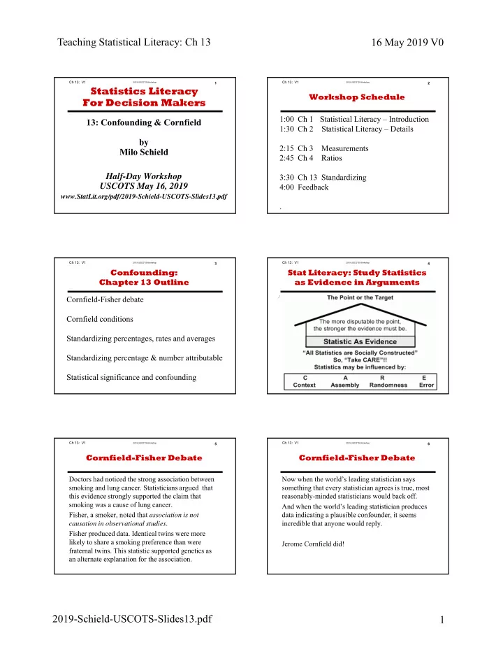
13: Confounding & Cornfield by Milo Schield Half-Day Workshop USCOTS May 16, 2019
www.StatLit.org/pdf/2019-Schield-USCOTS-Slides13.pdf
Statistics Literacy For Decision Makers
2019 USCOTS WorkshopCh 13: V1
1:00 Ch 1 Statistical Literacy – Introduction 1:30 Ch 2 Statistical Literacy – Details 2:15 Ch 3 Measurements 2:45 Ch 4 Ratios 3:30 Ch 13 Standardizing 4:00 Feedback .
2
Workshop Schedule
2019 USCOTS WorkshopCh 13: V1
Cornfield-Fisher debate Cornfield conditions Standardizing percentages, rates and averages Standardizing percentage & number attributable Statistical significance and confounding
3
Confounding: Chapter 13 Outline
2019 USCOTS WorkshopCh 13: V1 ./ 4
Stat Literacy: Study Statistics as Evidence in Arguments
2019 USCOTS WorkshopCh 13: V1
Doctors had noticed the strong association between smoking and lung cancer. Statisticians argued that this evidence strongly supported the claim that smoking was a cause of lung cancer. Fisher, a smoker, noted that association is not causation in observational studies. Fisher produced data. Identical twins were more likely to share a smoking preference than were fraternal twins. This statistic supported genetics as an alternate explanation for the association.
5
Cornfield-Fisher Debate
2019 USCOTS WorkshopCh 13: V1
Now when the world’s leading statistician says something that every statistician agrees is true, most reasonably-minded statisticians would back off. And when the world’s leading statistician produces data indicating a plausible confounder, it seems incredible that anyone would reply. Jerome Cornfield did!
6
Cornfield-Fisher Debate