
Statistical Literacy: Confounding 13 Jan, 2011 2011-Schield-UTSA-Confounding-Slides.pdf 1
UTSA Confounding 20111
MILO SCHIELD,
Augsburg College
Director, W. M. Keck Statistical Literacy Project Vice President, National Numeracy Network US Rep., International Statistical Literacy Project
January 13, 2011 University of Texas San Antonio (UTSA) Slides at www.StatLit.org/pdf/ 2011-Schield-UTSA-Confounding-Slides.pdf
Statistical Literacy: Confounding
20112
Statistical Literacy
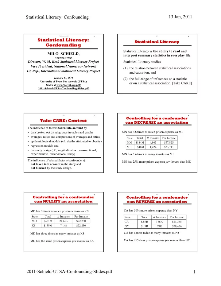
Statistical literacy is the ability to read and interpret summary statistics in everyday life. Statistical Literacy studies (1) the relation between statistical associations and causation, and (2) the full-range of influences on a statistic
- r on a statistical association. [Take CARE]
3
Take CARE: Context
The influence of factors taken into account by
- data broken out by subgroups in tables and graphs
- averages, ratios and comparisons of averages and ratios
- epidemiological models (cf., deaths attributed to obesity)
- regression models and
- the study design (cf., longitudinal vs. cross-sectional;
experiment vs. observational study). The influence of related factors (confounders) not taken into account in the study and not blocked by the study design.
20114
Controlling for a confounder can DECREASE an association
MN has 3.8 times as much prison expense as ME MN has 3.4 times as many inmates as ME MN has 25% more prison expense per inmate than ME State Total # Inmates Per Inmate MN $184M 4,865 $37,825 ME $48M 1,424 $33,711
20115
Controlling for a confounder can NULLIFY an association
MD has 3 times as much prison expense as KS MD has three times as many inmates as KS MD has the same prison expense per inmate as KS State Total # Inmates Per Inmate MD $481M 21,623 $22,250 KS $159M 7,148 $22,250
20116
Controlling for a confounder can REVERSE an association
CA has 50% more prison expense than NY CA has almost twice as many inmates as NY CA has 25% less prison expense per inmate than NY State Total # Inmates Per Inmate CA $2.9B 136K $21,385 NY $1.9B 69K $28,426