
IASE 2B: Teaching Confounding V0G 7/21/2016 www.StatLit.org/pdf/2016-Schield-IASE-Slides-2B.pdf Page 1
2016 IASEV0 1
Milo Schield, Augsburg College
Member: International Statistical Institute US Rep: International Statistical Literacy Project
- VP. National Numeracy Network
IASE Roundtable in Berlin
July 20, 2016
www.StatLit.org/pdf/2016-Schield-IASE-2Slides.pdf
B: Teaching Confounding and Multivariate Thinking
V0
2016 IASE-22
GAISE 2016: Two New Emphases
- a. Teach statistics as an investigative process of
problem-solving and decision making.
- Statistics is a problem-solving and decision-making
process, not a collection of formulas and methods.
- b. Give students experience in multivariable
thinking
- The world is a tangle of complex problems with inter-
related factors. Lets show students how to explore relationships among many variables
V0
2016 IASE-23
GAISE 2016 Add Multivariable Thinking
- give "students experience with multivariable thinking"
- understand “the possible impact of ... confounding"
- See how "a third variable can change our understanding"
- Help students "identify observational studies"
- teach multivariate thinking "in stages" and
- use "simple approaches (such as stratification)”
This change is HUGE! It may be the biggest content change since dropping combinations in the 1980s.
V0
2016 IASE-24
GAISE 2016 Appendix B: Observational Data Multivariable thinking is critical to make sense of the observational data around us. The real world is complex and can’t be described well by one or two
- variables. [Italics added]
V0
2016 IASE-25
GAISE 2016 Confounding “The 2014 ASA guidelines for undergraduate programs in statistics recommend that students
- btain a clear understanding of principles of
statistical design and tools to assess and account for the possible impact of other measured and unmeasured confounding variables (ASA, 2014).“
http://www.amstat.org/education/gaise/collegeupdate/GAISE2016_DRAFT.pdf
V0
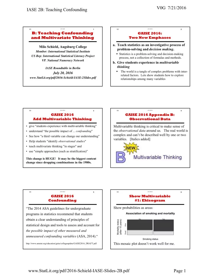
2016 IASE-26
Show Multivariable #1: Ekisogram Show probabilities as areas: This mosaic plot doesn’t work well for me.