v v 1 3 20 liquids through pipe 16 Vancouver parts through an - PDF document

4.2 Network Flows ◮ A directed graph can model a flow network where some material (e.g., widgets, current, . . . ) is produced or enters the network at Mat 3770 a source and is consumed at a sink . Network Flows ◮ Production and consumption are at a steady rate , which is the same for both. Spring 2014 ◮ The flow of the material at any point in the system is the rate at which the material moves through it. 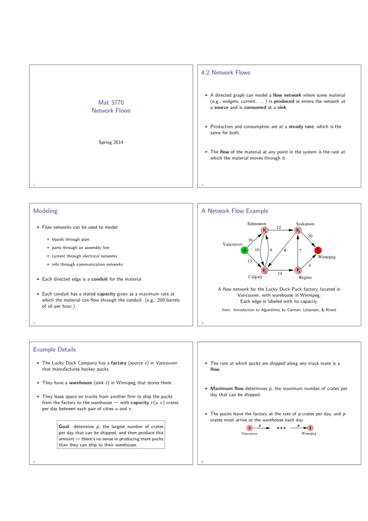1 2 Modeling A Network Flow Example Edmonton Saskatoon ◮ Flow networks can be used to model: 12 v v 1 3 20 ◮ liquids through pipe 16 Vancouver ◮ parts through an assembly line s t 10 4 9 7 ◮ current through electrical networks Winnipeg 13 ◮ info through communication networks 4 v v 4 2 14 Calgary Regina ◮ Each directed edge is a conduit for the material. A flow network for the Lucky Duck Puck factory, located in ◮ Each conduit has a stated capacity given as a maximum rate at Vancouver, with warehouse in Winnipeg. which the material can flow through the conduit. (e.g., 200 barrels Each edge is labeled with its capacity. of oil per hour.) from: Introduction to Algorithms , by Cormen, Leiserson, & Rivest 3 4 Example Details ◮ The Lucky Duck Company has a factory (source s ) in Vancouver ◮ The rate at which pucks are shipped along any truck route is a that manufactures hockey pucks. flow . ◮ They have a warehouse (sink t ) in Winnipeg that stores them. ◮ Maximum flow determines p , the maximum number of crates per day that can be shipped. ◮ They lease space on trucks from another firm to ship the pucks from the factory to the warehouse — with capacity c ( u , v ) crates per day between each pair of cities u and v . ◮ The pucks leave the factory at the rate of p crates per day, and p crates must arrive at the warehouse each day: Goal : determine p , the largest number of crates p p s t per day that can be shipped, and then produce this Vancouver Winnipeg amount — there’s no sense in producing more pucks than they can ship to their warehouse. 5 6

Flow Conservation ◮ Shipping time is not a concern, only the flow of p crates/day. ◮ Vertices are conduit junctions . Other than the source and sink , material flows through the vertices without collecting in them. ◮ Capacity constraints are given by the restriction that the flow f ( u , v ) from city u to city v be at most c ( u , v ) crates per day. ◮ Hence, the rate at which material enters a vertex must equal the rate at which it leaves the vertex. ◮ In a steady state , the number of crates entering and the number leaving an intermediate city must be equal. ◮ This property is called flow conservation , and is similar in concept to Kirchhoff’s Current Law concerning electrical current. 7 8 Maximum–flow Assumptions A flow network , G = (V, E), is a directed graph in which each edge (u, v) ∈ E has a non–negative capacity c(u, v) ≥ 0. The Maximum–flow problem is the simplest problem concerning flow networks: If (u, v) �∈ E, we assume c(u, v) = 0. What is the greatest rate at which material can ∀ x ∈ E, In( x ) and Out( x ) are the edges into and out of vertex x . be shipped from source to sink without violating any capacity constraints? The integer c( e ) associated with edge e is a capacity or upper bound. 9 10 Tucker: a–z (Source to Sink) Flow φ 12/12 v v ◮ An a–z flow φ in a directed network N is an integer–valued 1 3 15/20 function φ defined on each edge e . 11/16 ◮ φ ( e ) is the flow in e , together with a source vertex a and a sink s 4/9 10 t 1/4 7/7 vertex z satisfying the following three conditions: 8/13 1. Capacity Constraint: 0 ≤ φ ( e ) ≤ c( e ) 4/4 We don’t want backflow , nor to exceed any edge’s capacity v v 4 2 11/14 2. φ ( e ) = 0 if e ∈ IN(a) or e ∈ OUT(z) We want the flow to go from source to sink, not vice–versa A flow f with value | f | = 19. 3. Flow Conservation: Only positive net flows (crates shipped) are shown. For x � = a or z, � e ∈ IN ( x ) φ ( e ) = � e ∈ OUT ( x ) φ ( e ) If f ( u , v ) > 0, edge ( u , v ) is labeled by f ( u , v ) / c ( u , v ). For every vertex other than the source and sink, the flow into and If f ( u , v ) ≤ 0, edge ( u , v ) is labeled only by its capacity. out of that vertex must be equal 11 12

Flow Networks A flow in G is a real–valued function f : V × V → ℜ that satisfies ◮ The quantity f ( u , v ), which can be positive, negative, or zero, is the following three properties: called the flow from vertex u to vertex v . 1. Capacity constraint : the flow along an edge cannot exceed its capacity: ∀ u , v , ∈ V , f ( u , v ) ≤ c ( u , v ) ◮ The value of a flow f is defined as: | f | = � v ∈ V f ( s , v ) = � v ∈ V f ( v , t ). 2. Skew symmetry : the flow from a vertex u to a vertex v is the negative of the flow in the reverse direction: I.e., the total flow out of the source or into the sink . ∀ u , v ∈ V , f ( u , v ) = − f ( v , u ) ◮ In the maximum–flow problem , we are given a flow network G 3. Flow conservation : the net flow of a vertex (other than the with source s and sink t , and we wish to find a flow of maximum source or sink) is 0: value from s to t . � ∀ u ∈ V − { s , t } , f ( u , v ) = 0 v ∈ V 13 14 Flow In Equals Flow Out 1. The total positive flow entering a vertex v is defined by 1. (By skew symmetry) The flow from a vertex to itself is 0, since for all u ∈ V , we have f ( u , u ) = − f ( u , u ) � f ( u , v ) u ∈ V , f ( u , v ) > 0 2. (By skew symmetry) We can rewrite the flow–conservation 2. The total positive flow leaving a vertex v is defined by property as the total flow into a vertex is 0: � f ( v , u ) � ∀ v ∈ V − { s , t } , f ( u , v ) = 0 u ∈ V , f ( v , u ) > 0 u ∈ V 3. The positive net flow entering a vertex (other than the source or sink) must equal the positive net flow leaving the vertex. 15 16 Cancellation There can be no flow between u and v ◮ Cancellation allows us to represent the shipments between two if there is no edge between them. cities by a positive flow along at most one of the two edges between the corresponding vertices. If there is no edge between u and v , i.e., ( u , v ) �∈ E and ( v , u ) �∈ E , then: ◮ If there is zero or negative flow from one vertex to another, no shipments need be made in that direction. ◮ If there is no edge, then the capacity is zero. And by the Capacity Constraint, the flows must be ≤ 0. ◮ Any situation in which pucks are shipped in both directions c(u, v) = c(v, u) = 0 ⇒ f(u, v) ≤ 0, f(v, u) ≤ 0 between two cities can be transformed using cancellation into an equivalent situation in which pucks are shipped only in the ◮ By skew symmetry, the flow must be zero. direction of positive flow . f(u, v) = − f(v, u) ⇒ f(u, v) = f(v, u) = 0 ◮ No constraints are violated since the net flow between the two vertices is the same. 17 18

Cancellation in General Cancellation Example v v v v v 1 1 1 1 1 ◮ Suppose edge ( u , v ) has flow value f ( u , v ) 10 8/10 8/10 5/10 10 4 4 3/4 4 2/4 ◮ Now, increase the flow on the on edge ( v , u ) by some amount d v v v v v 2 2 2 2 2 (a) (b) (c) (d) (e) ◮ Mathematically, this operation must decrease f ( u , v ) by d (a) Vertices v 1 and v 2 , with c ( v 1 , v 2 ) = 10 and c ( v 2 , v 1 ) = 4 (b) Net flow when 8 crates per day are shipped from v 1 to v 2 . ◮ Conceptually, we can think of these d units as canceling d units (c) An additional shipment of 3 crates per day from v 2 to v 1 . of flow that are already on edge ( u , v ) (d) By canceling flow going in opposite directions, we can represent the situation in (c) with positive flow in one direction only. (e) Another 7 crates per day shipped from v 2 to v 1 results in a net of 2 crates per day from v 2 to v 1 . 19 20 Flow Cuts Cut Example 12/12 v v 1 3 15/20 ◮ A cut(S, T) of flow network G = (V, E), is a partition of V into 11/16 S and T = V - S, such that source ∈ S and sink ∈ T. 4/9 s 10 1/4 t 7/7 8/13 ◮ If f is a flow, then the net flow across the cut ( S , T ) is defined 4/4 v v to be f ( S , T ). 4 2 11/14 S T ◮ The capacity of the cut ( S , T ) is c ( S , T ). cut( { a, v 1 , v 2 } , { v 3 , v 4 , z } ) has net flow : f ( v 1 , v 3 ) + f ( v 2 , v 3 ) + F ( v 2 , v 4 ) = 12 − 4 + 11 = 19. And, its capacity is: c ( v 1 , v 3 ) + c ( v 2 , v 4 ) = 12 + 14 = 26. 21 22 Ford–Fulkerson Method Ford–Fulkerson Solution Each iteration will increase the flow until The Ford–Fulkerson Method for solving the maximum–flow the maximum is reached problem depends on three key concepts: 1. residual networks Ford-Fulkerson Method (G, s, t) initialize flow f to 0 2. augmenting paths while there exists an augmenting path p 3. cuts augment flow f along p return f 23 24