Overview of this module Course 02429 Analysis of correlated data: - - PowerPoint PPT Presentation

Course 02429 Analysis of correlated data: Mixed Linear Models Module 9: Random coefficient models Per Bruun Brockhoff

DTU Compute Building 324 - room 220 Technical University of Denmark 2800 Lyngby – Denmark e-mail: perbb@dtu.dk

Per Bruun Brockhoff (perbb@dtu.dk) Mixed Linear Models, Module 9 Fall 2014 1 / 20

Overview of this module

1

Random coefficient models, motivation Example: Constructed data The relevant models The mixed model Two-step regression analysis Testing the variance structure

2

Example: Consumer preference mapping of carrots Results

3

Perspectives

Per Bruun Brockhoff (perbb@dtu.dk) Mixed Linear Models, Module 9 Fall 2014 2 / 20 Random coefficient models, motivation

Content of Module 9:

Constructed data example Models and analysis:

Simple regression analysis Fixed effects analysis Two step analysis Random coefficients model

Example: Consumer preference mapping of carrots

Per Bruun Brockhoff (perbb@dtu.dk) Mixed Linear Models, Module 9 Fall 2014 4 / 20 Random coefficient models, motivation Example: Constructed data

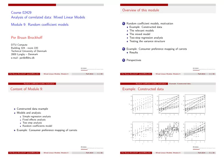
Example: Constructed data

2 4 6 8 10 10 15 20 25 x y1 2 4 6 8 10 10 15 20 25 x y1 2 4 6 8 10 10 15 20 25 x y1 2 4 6 8 10 5 10 15 20 25 x y2 2 4 6 8 10 5 10 15 20 25 x y2 2 4 6 8 10 5 10 15 20 25 x y2

Per Bruun Brockhoff (perbb@dtu.dk) Mixed Linear Models, Module 9 Fall 2014 5 / 20

Random coefficient models, motivation The relevant models

Models

The simple regression model: yj = α + βxj + ǫj Different FIXED regression lines: yi = α(subjecti) + β(subjecti)xi + ǫi Different RANDOM regression lines: yi = a(subjecti) + b(subjecti)xi + ǫi where a(k) ∼ N(α, σ2

a), b(k) ∼ N(β, σ2 b), ǫi ∼ N(0, σ2)

Per Bruun Brockhoff (perbb@dtu.dk) Mixed Linear Models, Module 9 Fall 2014 6 / 20 Random coefficient models, motivation The mixed model

A mixed model

Splitting the mean and variance structure: yi = α + βxi + a(subjecti) + b(subjecti)xi + ǫi a(k) ∼ N(0, σ2

a), b(k) ∼ N(0, σ2 b), ǫi ∼ N(0, σ2)

Or slightly more general: (a(k), b(k)) ∼ N(0, σ2

a

σab σab σ2

b

• ), ǫi ∼ N(0, σ2)

Allowing for correlation between between intercepts and slopes.

Per Bruun Brockhoff (perbb@dtu.dk) Mixed Linear Models, Module 9 Fall 2014 7 / 20 Random coefficient models, motivation Two-step regression analysis

Two-step regression analysis – constructed data

For “nice“ data sets (like the constructed data): Random coefficient regression corresponds to two-step analysis:

1

Carry out a regression analysis for each subject.

2

Do subsequent calculations on the parameter estimates from these regression analyzes to obtain the average slope (and intercept) and their standard errors.

Results: Data set 1 Data set 2 α β α β Average 10.7279 0.9046 7.8356 1.2152 SE 1.2759 0.1570 0.9255 0.1460 Lower 7.8416 0.5495 5.7419 0.8850 Upper 13.6142 1.2597 9.9293 1.5454 NB: These are the (fixed effects) results from the random coefficient model.

Per Bruun Brockhoff (perbb@dtu.dk) Mixed Linear Models, Module 9 Fall 2014 8 / 20 Random coefficient models, motivation Two-step regression analysis

Constructed data, cont.

Observed variances for slopes (two-step): Data set 1: s2

ˆ β = 0.2465

Data set 2: s2

ˆ β = 0.2130

Estimated variance components (Random coefficient model): Data set 1: ˆ σ2

b = 0.2456, ˆ

σ2 = 0.0732 and for data set 2: Data set 2: ˆ σ2

b = 0.021, ˆ

σ2 = 17.07

Per Bruun Brockhoff (perbb@dtu.dk) Mixed Linear Models, Module 9 Fall 2014 9 / 20

Random coefficient models, motivation Two-step regression analysis

Example: Constructed data

2 4 6 8 10 10 15 20 25 x y1 2 4 6 8 10 10 15 20 25 x y1 2 4 6 8 10 10 15 20 25 x y1 2 4 6 8 10 5 10 15 20 25 x y2 2 4 6 8 10 5 10 15 20 25 x y2 2 4 6 8 10 5 10 15 20 25 x y2

Per Bruun Brockhoff (perbb@dtu.dk) Mixed Linear Models, Module 9 Fall 2014 10 / 20 Random coefficient models, motivation Testing the variance structure

Notes

Random coefficent models tells the proper story about the data Two-step procedure only strictly valid in certain nice cases It is possible to test the equal slopes hypothesis: H0 : σ2

b = 0

By the REML likelihood test: G = −2lREML,1 − (−2lREML,2) Data set 2, NON-significant: G = −2lREML,1 − (−2lREML,2) = 0.65 Data set 1, EXTREMELY significant: G = −2lREML,1 − (−2lREML,2) = 249.9

Per Bruun Brockhoff (perbb@dtu.dk) Mixed Linear Models, Module 9 Fall 2014 11 / 20 Example: Consumer preference mapping of carrots

Example: Consumer preference mapping of carrots

[I]1122

1236

[cons]102

103

prod11

12

size1

2

01

1

Factors:

103 consumers in 2 groups (Homesize) 12 carrot products

Y-data: Preference scores X-data: Sensory measurements on the products. Aim: Study average relationships between preference and 2 sensory score variables . Starting model, FIXED part:

Homesize, average intercepts and slopes depending on homesize.

Starting model, RANDOM part:

Random regression coefficients on the two sensory variables. Random product effect

Per Bruun Brockhoff (perbb@dtu.dk) Mixed Linear Models, Module 9 Fall 2014 13 / 20 Example: Consumer preference mapping of carrots Results

Significance testing approach

1 Simplify the variance part of the model

(G statistics)

2 Then simplify the fixed/systematic structure

(Table of F-tests of fixed effects) Results, final model: yi = α(sizei) + β2 · sens2i + a(consi) +b2(consi) · sens2i + d(prodi) + ǫi where a(k) ∼ N(0, σ2

a), b2(k) ∼ N(0, σ2 b2), k = 1, . . . 103.

and d(prodi) ∼ N(0, σ2

P ), ǫi ∼ N(0, σ2)

Per Bruun Brockhoff (perbb@dtu.dk) Mixed Linear Models, Module 9 Fall 2014 14 / 20

Example: Consumer preference mapping of carrots Results

Results

The variance part:

No significant variation in sens1 coefficients. Significant variation in sens2 coefficients. Significant (additional) product variation. No significant correlation between sens2 intercepts and slopes.

Estimates - all parameters: ˆ σb2 0.0545 ˆ σa 0.442 ˆ σP 0.1774 ˆ σ 1.0194 ˆ α(Homesize1) 4.91 ˆ α(Homesize3) 4.67 ˆ β2 0.071

Per Bruun Brockhoff (perbb@dtu.dk) Mixed Linear Models, Module 9 Fall 2014 15 / 20 Example: Consumer preference mapping of carrots Results

Results

Confidence intervals: 2.5 % 97.5 % .sig01 0.03 0.08 .sig02 0.36 0.53 .sig03 0.09 0.29 .sigma 0.98 1.07 Homesize1 4.74 5.08 Homesize3-Homesize1

• 0.45
• 0.03

sens2 0.04 0.10

Per Bruun Brockhoff (perbb@dtu.dk) Mixed Linear Models, Module 9 Fall 2014 16 / 20 Example: Consumer preference mapping of carrots Results

Results, fixed part

No relation of preference to sens1. Significant relation to sens2 (sweetness): ˆ β2 = 0.071, [0.04, 0.10] The homesize story: ˆ α(1) + ˆ β2 · sens2 = 4.91, [4.73, 5.09] ˆ α(2) + ˆ β2 · sens2 = 4.67, [4.47, 4.85] ˆ α(1) − ˆ α(2) = 0.25, [0.04, 0.46] Homes with more persons tend to have a slightly lower preference in general for such carrot products.

Per Bruun Brockhoff (perbb@dtu.dk) Mixed Linear Models, Module 9 Fall 2014 17 / 20 Perspectives

Random coefficient models in perspective

Random extensions of regression and/or ANCOVA models. Relevant for hierarchical/clustered data. Also relevant for repeated measures data. Can be directly extended to polynomial structures. Can extend with residual correlation structures. May enter as components of any kind of analysis.

Per Bruun Brockhoff (perbb@dtu.dk) Mixed Linear Models, Module 9 Fall 2014 19 / 20

Perspectives

Overview of this module

1

Random coefficient models, motivation Example: Constructed data The relevant models The mixed model Two-step regression analysis Testing the variance structure

2

Example: Consumer preference mapping of carrots Results

3

Perspectives

Per Bruun Brockhoff (perbb@dtu.dk) Mixed Linear Models, Module 9 Fall 2014 20 / 20