
SLIDE 1
An observable random vector X of dimension p has mean vector and covariance matrix Σ Factor rotation (cf. section 9.4 )
− = + X
- LF
ε
We consider the factor model
1
( ) Cov( ) ( ) E E = ′ = = F F FF I
where
1 2
( ) Cov( ) ( ) diag{ , , , }
p
E E ψ ψ ψ = ′ = = = ε ε εε Ψ … Cov( , ) = ε F
The model implies that
cov( ) {( )( ) } E ′ = = − − Σ X X X
- ′
= + LL Ψ
In particular:
Var( ) X σ =
2
Var( )
ii i
X σ =
2 1 m ij i j
l ψ
=
= +
∑
2
communality specific variance (uniqueness)
i i
h ψ = +
- If T is a m x m orthogonal matrix, the factor model may be
reformulated as
− = + X
- LF
ε
where
* *
and ′ = = L LT F T F ′ = + LTT F ε
* *
= + L F ε
The covariance matrix remains unchanged:
′+ LL Ψ ′ ′ = + LTT L Ψ
* *′
= + L L Ψ
3
Thus it is impossible on the basis of observations to distinguish the loadings L from the loadings L*, so the factor loadings L are determined only up to an
- rthogonal matrix T (corresponding to a rotation)
′+ LL Ψ ′ ′ = + LTT L Ψ
* *′
= + L L Ψ
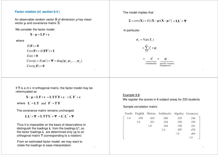
From an estimated factor model, we may want to rotate the loadings to ease interpretation Example 9.8: We register the scores in 6 subject areas for 220 students Sample correlation matrix
4