Overview of this module Course 02429 Analysis of correlated data: - - PowerPoint PPT Presentation

Course 02429 Analysis of correlated data: Mixed Linear Models Module 12: Repeated measures II, advanced methods Per Bruun Brockhoff

DTU Compute Building 324 - room 220 Technical University of Denmark 2800 Lyngby – Denmark e-mail: perbb@dtu.dk

Per Bruun Brockhoff (perbb@dtu.dk) Mixed Linear Models, Module 12 Fall 2014 1 / 24 Overview of this module

Overview of this module

1

Different view on the random effects approach Example: Activity of rats

2

Gaussian model of spatial correlation Example: Activity of rats

3

Other spatial correlation structures

4

Diagram of analysis

5

The semi-variogram

6

Analysing the time structure by polynomial regression

Per Bruun Brockhoff (perbb@dtu.dk) Mixed Linear Models, Module 12 Fall 2014 2 / 24 Aim of this module

Aim of this module

Extend the toolbox for dealing with repeated measures Introduce models where the covariance structure is directly specified Improve our ability to handle long series See how to specify these models in R

Per Bruun Brockhoff (perbb@dtu.dk) Mixed Linear Models, Module 12 Fall 2014 3 / 24 Aim of this module

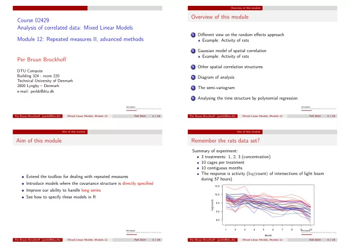
Remember the rats data set?

Summary of experiment: 3 treatments: 1, 2, 3 (concentration) 10 cages per treatment 10 contiguous months The response is activity (log(count) of intersections of light beam during 57 hours)

Month log(count) 8.5 9.0 9.5 10.0 10.5 1 2 3 4 5 6 7 8 9 10 Per Bruun Brockhoff (perbb@dtu.dk) Mixed Linear Models, Module 12 Fall 2014 4 / 24

Different view on the random effects approach

Different view on the random effects approach

Any mixed model can be expressed as: y ∼ N(Xβ, ZGZ′ + R), The total covariance of all observations are described by V = ZGZ′ + R The ZGZ′ part is specified through the random effects of the model The R part has so far been σ2I, but in this module we will put some structure into R For instance the structure known from the random effects model

cov(yi1, yi2) =    , if individuali1 = individuali2 and i1 = i2 σ2

individual

, if individuali1 = individuali2 and i1 = i2 σ2

individual + σ2

, if i1 = i2

This structure is known as compound symmetry

Per Bruun Brockhoff (perbb@dtu.dk) Mixed Linear Models, Module 12 Fall 2014 6 / 24 Different view on the random effects approach Example: Activity of rats

Activity of rats analyzed via compound symmetry model

The model is the same as the random effects model, but specified directly lnc ∼ N(µ, V), where µi = µ + α(treatmi) + β(monthi) + γ(treatmi, monthi), and Vi1,i2 =    , if cagei1 = cagei2 and i1 = i2 σ2

d

, if cagei1 = cagei2 and i1 = i2 σ2

d + σ2

, if i1 = i2 Implemented in R traditionally by a random effect:

lme(lnc ~ month + treatm + month:treatm, random = ~1 | cage, data = rats)

OR directly into the R-matrix:

gls(lnc~month+treatm+month:treatm, correlation=corCompSymm(form=~1|cage),data=rats)

Per Bruun Brockhoff (perbb@dtu.dk) Mixed Linear Models, Module 12 Fall 2014 7 / 24 Gaussian model of spatial correlation

Gaussian model of spatial correlation

Covariance structures depending on “how far” observations are apart are known as spatial The following covariance structure has been proposed for repeated measurements

Vi1,i2 =        , if individual i1 = individual i2 and i1 = i2 ν2 + τ 2 exp

• −(ti1 −ti2 )2

ρ2

• , if individual i1 = individual i2 and i1 = i2

ν2 + τ 2 + σ2 , if i1 = i2 Distance ti1 − ti2 Covariance 0.83ρ ν2 ν2 + τ2 ν2 + 0.5τ2

Per Bruun Brockhoff (perbb@dtu.dk) Mixed Linear Models, Module 12 Fall 2014 9 / 24 Gaussian model of spatial correlation Example: Activity of rats

Rats data via spatial Gaussian correlation model

The entire model is:

lnc ∼ N(µ, V), where µi = µ + α(treatmi) + β(monthi) + γ(treatmi, monthi), and Vi1,i2 =        , if cagei1 = cagei2 and i1 = i2 ν2 + τ 2 exp

• −(monthi1 −monthi2 )2

ρ2

• , if cagei1 = cagei2 and i1 = i2

ν2 + τ 2 + σ2 , if i1 = i2

This model is implemented by:

lme(lnc~month+treatm+month:treatm, random=~1|cage, correlation=corGaus(form=~as.numeric(month)|cage,nugget=T), data=rats)

Per Bruun Brockhoff (perbb@dtu.dk) Mixed Linear Models, Module 12 Fall 2014 10 / 24

Gaussian model of spatial correlation Example: Activity of rats

The relevant part of the R output is:

Random effects: Formula: ~1 | cage (Intercept) Residual StdDev: 0.1404056 (= ˆ ν) 0.2171559 (= √ ˆ σ2 + ˆ τ 2) Correlation Structure: Gaussian spatial correlation Formula: ~as.numeric(month) | cage Parameter estimate(s): range nugget 2.3863954 (= ˆ ρ2) 0.2186744 (= ˆ σ2/(ˆ σ2 + ˆ τ 2)) Number of Observations: 300 Number of Groups: 30

Notice the R parametrization of the variance parameters

Per Bruun Brockhoff (perbb@dtu.dk) Mixed Linear Models, Module 12 Fall 2014 11 / 24 Gaussian model of spatial correlation Example: Activity of rats

Reduction from spatial Gaussian to random effects?

The spatial Gaussian model (A) is an extension of the random effects model (B) Use the restricted/residual likelihood ratio test GA→B = 2ℓ(B)

re − 2ℓ(A) re , where GA→B ∼ χ2 2

For the rats data we get:

Model 2ℓre G–value df P–value (A) Spatial Gaussian

• 105.3

GA→B = 113.9 2 PA→B < 0.0001 (B) Random effects 8.6

The spatial Gaussian structure is clearly a better description of the covariance structure in the rats data set

Per Bruun Brockhoff (perbb@dtu.dk) Mixed Linear Models, Module 12 Fall 2014 12 / 24 Other spatial correlation structures

Other spatial correlation structures

R has several build–in correlation structures. A few examples are:

Write in R Name Correlation term corGaus Gaussian τ 2 exp{

−(ti1 −ti2 )2 ρ2

} corExp exponential τ 2 exp{

−|ti1 −ti2 | ρ

} corAR1 autoregressive(1) τ 2ρ|i1−i2| corSymm unstructured τ 2

i1,i2

Unfortunately is can be very difficult to choose — especially for “short” individual series General advice:

Keep it simple: Numerical problems often occur with (too) complicated structures Graphical methods: Especially for “long” series the (semi)–variogram is useful Information criteria: AIC or BIC = “2ℓ + penalty(#par)” can be used as guideline Try to cross–validate your main conclusion(s) by one of the “simple” methods

Per Bruun Brockhoff (perbb@dtu.dk) Mixed Linear Models, Module 12 Fall 2014 14 / 24 Diagram of analysis

Diagram of analysis

Select covariance structure from

knowledge about the experiment guided by information criteria

Covariance parameters are tested by likelihood ratio test The green arrow is often omitted by the argument that a non–significant simplification of the mean structure should not change the covariance structure much

Identify "individuals" Select fixed effects Select covariance structure Test covariance parameters Test fixed effects Interpret results Change model Change model Per Bruun Brockhoff (perbb@dtu.dk) Mixed Linear Models, Module 12 Fall 2014 16 / 24

The semi-variogram

The semi-variogram

Plotting of the empirical covariation (of residuals) versus "time" Plot of σ2 + γ(u), where

γ(u) = τ 2 1 − λ(u)

• λ(u) = exp{−u2/ρ2}

1 2 3 4 1 2 3 4 Time difference Covariance σ2 τ2 ν2

Per Bruun Brockhoff (perbb@dtu.dk) Mixed Linear Models, Module 12 Fall 2014 18 / 24 The semi-variogram

The semi-variogram

print(plot(Variogram(model2, form =˜as.numeric(month)|cage, data = rats)))

Distance Semivariogram

• 0.0

0.5 1.0 2 4 6 8

Per Bruun Brockhoff (perbb@dtu.dk) Mixed Linear Models, Module 12 Fall 2014 19 / 24 The semi-variogram

The semi-variogram

model3 <- lme(lnc month + treatm + month:treatm, random = 1 | cage, correlation = corExp(form =˜as.numeric(month) | cage, nugget = T), data = rats) print(plot(Variogram(model3, form =˜as.numeric(month)|cage, data = rats)))

Distance Semivariogram

• 0.0

0.2 0.4 0.6 0.8 1.0 2 4 6 8 Per Bruun Brockhoff (perbb@dtu.dk) Mixed Linear Models, Module 12 Fall 2014 20 / 24 The semi-variogram

The semi-variogram

model4 <- lme(lnc month + treatm + month:treatm, random = 1 | cage, correlation = corAR1(form = as.numeric(month) | cage), data = rats) print(plot(Variogram(model4, form =˜as.numeric(month)|cage, data = rats)))

Distance Semivariogram

0.2 0.4 0.6 0.8 1.0 2 4 6 8

• Per Bruun Brockhoff (perbb@dtu.dk)

Mixed Linear Models, Module 12 Fall 2014 21 / 24

Analysing the time structure by polynomial regression

Analysing the time structure by polynomial regression

1 Do the factor based analysis as shown above. 2 Explorative plotting of individual and treatment average regression

lines/curves.

3 Potentially make a ”high degree” decomposition based on the simple

”split-plot” repeated measures model using lmer and lmerTest.

4 Check if a linear or quadratic regression model could be used as an

alternative to the factor based model

5 IF a regression approach seems to capture what is going on, then try

to fit the random coefficient model as an alternativ to the correlation structure used from above - chose the best one at the end.

6 A possibility is that a factor based model is needed for the main effect

• f time, whereas a quantitative model would fit the interaction effect.

Per Bruun Brockhoff (perbb@dtu.dk) Mixed Linear Models, Module 12 Fall 2014 23 / 24 Analysing the time structure by polynomial regression

Overview of this module

1

Different view on the random effects approach Example: Activity of rats

2

Gaussian model of spatial correlation Example: Activity of rats

3

Other spatial correlation structures

4

Diagram of analysis

5

The semi-variogram

6

Analysing the time structure by polynomial regression

Per Bruun Brockhoff (perbb@dtu.dk) Mixed Linear Models, Module 12 Fall 2014 24 / 24