Overview of this module Course 02429 Analysis of correlated data: - - PowerPoint PPT Presentation

Course 02429 Analysis of correlated data: Mixed Linear Models Module 3: Drying of beech wood - a case study, part I Per Bruun Brockhoff

DTU Compute Building 324 - room 220 Technical University of Denmark 2800 Lyngby – Denmark e-mail: perbb@dtu.dk

Per Bruun Brockhoff (perbb@dtu.dk) Mixed Linear Models, Module 3 Fall 2014 1 / 26

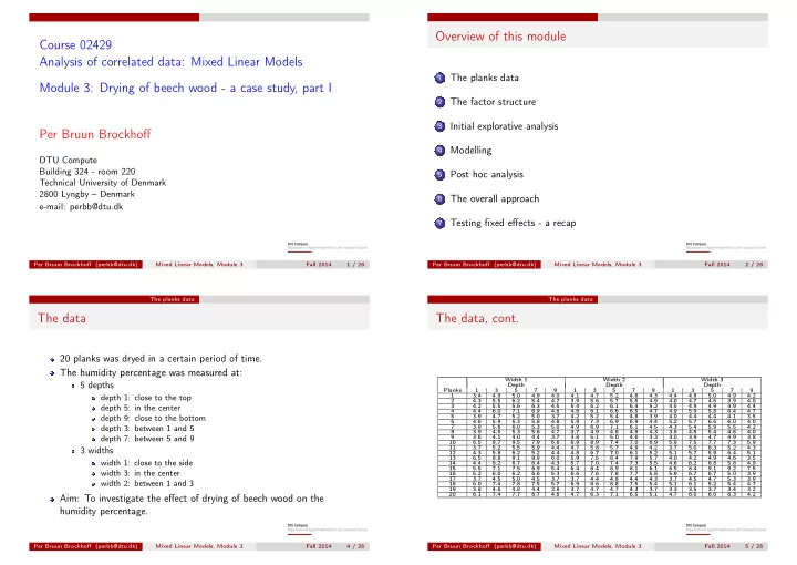
Overview of this module

1

The planks data

2

The factor structure

3

Initial explorative analysis

4

Modelling

5

Post hoc analysis

6

The overall approach

7

Testing fixed effects - a recap

Per Bruun Brockhoff (perbb@dtu.dk) Mixed Linear Models, Module 3 Fall 2014 2 / 26 The planks data

The data

20 planks was dryed in a certain period of time. The humidity percentage was measured at:

5 depths

depth 1: close to the top depth 5: in the center depth 9: close to the bottom depth 3: between 1 and 5 depth 7: between 5 and 9

3 widths

width 1: close to the side width 3: in the center width 2: between 1 and 3

Aim: To investigate the effect of drying of beech wood on the humidity percentage.

Per Bruun Brockhoff (perbb@dtu.dk) Mixed Linear Models, Module 3 Fall 2014 4 / 26 The planks data

The data, cont.

Width 1 Width 2 Width 3 Depth Depth Depth Planks 1 3 5 7 9 1 3 5 7 9 1 3 5 7 9 1 3.4 4.9 5.0 4.9 4.0 4.1 4.7 5.2 4.6 4.3 4.4 4.8 5.0 4.9 4.2 2 4.3 5.5 6.2 5.4 4.7 3.9 5.6 5.7 5.5 4.9 4.0 4.7 4.5 3.9 4.0 3 4.2 5.5 5.6 6.3 4.5 5.4 6.2 6.1 6.4 5.2 4.5 4.9 4.9 4.9 4.4 4 4.4 6.0 7.1 6.9 4.6 4.6 6.1 6.6 6.5 4.7 4.9 5.9 5.8 6.4 4.7 5 3.9 4.7 5.2 5.0 3.7 4.2 5.2 5.4 4.8 3.9 4.0 4.4 4.4 4.1 3.5 6 4.6 5.9 6.3 5.8 4.8 5.9 7.3 6.9 6.9 4.4 5.2 5.7 6.6 6.0 4.0 7 3.9 5.6 6.0 5.3 5.0 4.9 6.9 7.1 6.1 4.5 4.3 5.4 5.9 5.5 4.2 8 3.9 4.5 5.3 5.6 4.7 3.7 4.9 4.8 4.9 4.3 3.8 4.5 5.4 4.8 4.0 9 3.6 4.1 4.0 4.4 3.7 3.8 5.1 5.0 4.6 3.3 3.0 3.9 4.7 4.9 3.8 10 6.5 8.7 9.5 7.9 6.6 6.9 8.9 7.4 7.0 6.9 5.8 7.5 7.7 7.3 5.9 11 3.7 5.2 5.5 5.9 4.4 4.7 5.8 5.7 4.9 4.2 3.7 5.0 6.3 5.2 4.3 12 4.3 5.8 6.2 5.2 4.4 4.8 6.7 7.0 6.1 5.2 5.1 5.7 5.9 6.4 5.1 13 6.5 8.8 9.1 8.9 6.0 5.9 7.5 8.4 7.9 5.7 4.0 4.2 4.9 4.6 3.5 14 4.4 6.2 6.7 6.4 4.3 5.7 7.0 7.4 7.3 5.5 4.6 6.2 6.8 5.8 4.9 15 5.5 7.1 7.5 6.9 5.4 6.4 8.4 8.9 8.1 6.1 6.5 8.4 9.1 9.2 7.5 16 5.2 6.0 6.2 6.6 5.3 6.6 7.6 7.8 7.7 5.8 5.9 6.7 6.7 5.0 3.9 17 3.7 4.5 5.0 4.5 3.7 3.7 4.4 4.8 4.4 4.3 3.7 4.5 4.7 5.3 3.9 18 6.0 7.4 7.8 7.5 5.7 6.9 8.6 8.8 7.5 5.4 5.1 6.1 5.2 5.4 4.7 19 3.8 4.6 4.8 4.4 3.8 3.7 4.7 4.7 4.3 3.7 3.3 3.5 3.7 3.4 3.2 20 6.1 7.4 7.7 6.7 4.6 4.7 6.3 7.1 6.5 5.1 4.7 6.0 6.0 6.3 4.2 Per Bruun Brockhoff (perbb@dtu.dk) Mixed Linear Models, Module 3 Fall 2014 5 / 26

The factor structure

Identify the factors and their structure

Factors:

I: 300 experimental units 0: 1 overall level depth: 5 levels width: 3 levels plank: 20 levels Crossed "treatment" structure: width × depth: 15 levels

plank is a natural block effect.

Per Bruun Brockhoff (perbb@dtu.dk) Mixed Linear Models, Module 3 Fall 2014 7 / 26 The factor structure

Identify the factors and their structure, cont.

Factor structure:

[I]266

300

depth × width8

15

[plank]19

20

width2

3

depth4

5

01

1

Model: Yi = µ+α(widthi)+β(depthi)+γ(widthi, depthi)+d(planki)+ǫi, d(j) ∼ N(0, σ2

Plank), ǫi ∼ N(0, σ2).

j = 1, . . . , 20, i = 1, . . . , 300 (A larger model is introduced in Module4 (and Module6), but let us do as if we didn’t see that yet)

Per Bruun Brockhoff (perbb@dtu.dk) Mixed Linear Models, Module 3 Fall 2014 8 / 26 Initial explorative analysis

Initial explorative analysis - boxplots

4 5 6 7 8 width mean of humidity 1 2 3 4 5 6 7 8 depth mean of humidity 1 3 5 7 9 4.5 5.0 5.5 6.0 6.5 mean of humidity 1 2 3 4.5 5.0 5.5 6.0 6.5 mean of humidity 1 3 5 7 9 Per Bruun Brockhoff (perbb@dtu.dk) Mixed Linear Models, Module 3 Fall 2014 10 / 26 Initial explorative analysis

Initial explorative analysis - boxplots

• 1

2 3 3 4 5 6 7 8 9

• 1

3 5 7 9 3 4 5 6 7 8 9

• 1

4 7 10 14 18 3 4 5 6 7 8 9

• 1.1

1.3 1.5 1.7 1.9 3 4 5 6 7 8 9 Per Bruun Brockhoff (perbb@dtu.dk) Mixed Linear Models, Module 3 Fall 2014 11 / 26

Modelling

Test of overall effects/model reduction

Fixed effects ANOVA tables: Source of Numerator Denominator Sums of Mean variation degrees degrees squares squares

• f freedom
• f freedom

depth 4 266 78.26 <0.0001 width 2 266 29.65 <0.0001 depth*width 8 266 1.08 0.3745 Source of Numerator Denominator Sums of Mean variation degrees degrees squares squares

• f freedom
• f freedom

depth 4 274 78.07 <0.0001 width 2 274 29.57 <0.0001

Per Bruun Brockhoff (perbb@dtu.dk) Mixed Linear Models, Module 3 Fall 2014 13 / 26 Modelling

Final model

[I]274

300

[plank]19

20

width2

3

depth4

5

01

1

Corresponding to; Yi = µ + α(widthi) + β(depthi) + d(planki) + ǫi d(j) ∼ N(0, σ2

Plank), ǫijk ∼ N(0, σ2).

Per Bruun Brockhoff (perbb@dtu.dk) Mixed Linear Models, Module 3 Fall 2014 14 / 26 Post hoc analysis

Post hoc analysis and summarizing the results

Estimates of the variance parameters: ˆ σ2

Planks = 0.979,

ˆ σ2 = 0.636 ˆ σPlanks = 0.990, ˆ σ = 0.4047 2.5 % 97.5 % .sig01 0.72 1.37 .sigma 0.58 0.69

Per Bruun Brockhoff (perbb@dtu.dk) Mixed Linear Models, Module 3 Fall 2014 16 / 26 Post hoc analysis

Post hoc analysis and summarizing the results

Estimates of the fixed parameters: Parameter Estimate SE Lower Upper Depth 1 µ + β(1) 4.7150 0.2361 4.2270 5.2030 Depth 3 µ + β(2) 5.9050 0.2361 5.4170 6.3930 Depth 5 µ + β(3) 6.1950 0.2361 5.7070 6.6830 Depth 7 µ + β(4) 5.8633 0.2361 5.3753 6.3514 Depth 9 µ + β(5) 4.6533 0.2361 4.1653 5.1414 Parameter Estimate SE Lower Upper Width 1 µ + α(1) 5.5140 0.2303 5.0352 5.9928 Width 2 µ + α(2) 5.7860 0.2303 5.3072 6.2648 Width 3 µ + α(3) 5.0990 0.2303 4.6202 5.5778

Per Bruun Brockhoff (perbb@dtu.dk) Mixed Linear Models, Module 3 Fall 2014 17 / 26

Post hoc analysis

Comparisons of the fixed parameters

t-test: t = ˆ β(1) − ˆ β(2) SE

• ˆ

β(1) − ˆ β(2)

• 95% confidence interval:

ˆ β(1) − ˆ β(2) ± t.975,274SE

• ˆ

β(1) − ˆ β(2)

• Warning: ONLY make comparisons decided for in advance (before

seeing the data) this way. For multiple comparisons between all levels of a factor: Use an "adjustment" method:

Bonferroni Tukey-Kramer Or other methods

Per Bruun Brockhoff (perbb@dtu.dk) Mixed Linear Models, Module 3 Fall 2014 18 / 26 Post hoc analysis

Comparisons of the fixed parameters, results

Depth Parameter Estimate SE Lower Upper P-value difference 1-3 β(1) − β(2)

• 1.1900

0.1162

• 1.5090
• 0.8710

<0.0001 1-5 β(1) − β(3)

• 1.4800

0.1162

• 1.7990
• 1.1610

<0.0001 1-7 β(1) − β(4)

• 1.1483

0.1162

• 1.4673
• 0.8294

<0.0001 1-9 β(1) − β(5) 0.06167 0.1162

• 0.2573

0.3806 0.9841 3-5 β(2) − β(3)

• 0.2900

0.1162

• 0.6090

0.02896 0.0943 3-7 β(2) − β(4) 0.04167 0.1162

• 0.2773

0.3606 0.9964 3-9 β(2) − β(5) 1.2517 0.1162 0.9327 1.5706 <0.0001 5-7 β(3) − β(4) 0.3317 0.1162 0.01271 0.6506 0.0370 5-9 β(3) − β(5) 1.5417 0.1162 1.2227 1.8606 <0.0001 7-9 β(4) − β(5) 1.2100 0.1162 0.8910 1.5290 <0.0001 Width Parameter Estimate SE Lower Upper P-value difference 1-2 α(1) − α(2)

• 0.2720

0.08997

• 0.4840
• 0.05998

0.0077 1-3 α(1) − α(3) 0.4150 0.08997 0.2030 0.6270 <0.0001 2-3 α(2) − α(3) 0.6870 0.08997 0.4750 0.8990 <0.0001

Per Bruun Brockhoff (perbb@dtu.dk) Mixed Linear Models, Module 3 Fall 2014 19 / 26 Post hoc analysis

Comparisons of the fixed parameters, in summary

Estimate Depth 9 4.6533a Depth 1 4.7150a Depth 7 5.8633b Depth 3 5.9050bc Depth 5 6.1950c Estimate Width 3 5.0990a Width 1 5.5140b Width 2 5.7860c

Per Bruun Brockhoff (perbb@dtu.dk) Mixed Linear Models, Module 3 Fall 2014 20 / 26 The overall approach

The overall approach - REALLY:

Identify factors and their structure leading to starting model. Explorative analysis Decide on which effects to be random (consider if residual error structure is needed) FIRST: Test of RANDOM effects/model reduction leading to final RANDOM model part

REML based test (always OK) or: ML based test (always OK) or: F-tests coming from a model where a random effect is considered fixed (sometimes OK) NOTE: Sometimes this part is skipped because the structure is simple. E.g. for the planks data!

THEN: Test of FIXED effects/model reduction of leading to final model Post hoc analysis of fixed effects (as before) Model Diagnostics is still missing: (Module 6)

Per Bruun Brockhoff (perbb@dtu.dk) Mixed Linear Models, Module 3 Fall 2014 22 / 26

Testing fixed effects - a recap

Testing fixed effects - a recap:

We generally always use the REML approach for the mixed model fit and variance part. (Allthough ML would be OK too) We estimate the fixed effects using the REML (but ML would be OK too) We construct F-statistics based on the REML (but ML would be OK too) WARNING: So although we say that "we use REML" for everything, there is ONE thing this does NOT mean:

NEVER compare the REML based fits for two models with DIFFERENT fixed effects structure. So: Never do a REML likelihood based test comparison of two different fixed effects models.

Per Bruun Brockhoff (perbb@dtu.dk) Mixed Linear Models, Module 3 Fall 2014 24 / 26 Testing fixed effects - a recap

Testing fixed effects - a recap:

So NEVER do:

model1 <- lmer(humidity depth*width +(1 | plank), data = planks) model2 <- lmer(humidity depth + width + (1 | plank), data = planks) anova(model1, model2, refit = FALSE)

whereas the following would be OK:(Since R would then do ML instead)

anova(model1, model2)

But we do not need this, since we use the F-statistics

Per Bruun Brockhoff (perbb@dtu.dk) Mixed Linear Models, Module 3 Fall 2014 25 / 26 Testing fixed effects - a recap

Overview of this module

1

The planks data

2

The factor structure

3

Initial explorative analysis

4

Modelling

5

Post hoc analysis

6

The overall approach

7

Testing fixed effects - a recap

Per Bruun Brockhoff (perbb@dtu.dk) Mixed Linear Models, Module 3 Fall 2014 26 / 26