Overview of this module Course 02429 Analysis of correlated data: - - PowerPoint PPT Presentation

Course 02429 Analysis of correlated data: Mixed Linear Models Module 11: Repeated measures I, simple methods Per Bruun Brockhoff

DTU Compute Building 324 - room 220 Technical University of Denmark 2800 Lyngby – Denmark e-mail: perbb@dtu.dk

Per Bruun Brockhoff (perbb@dtu.dk) Mixed Linear Models, Module 11 Fall 2014 1 / 18 Overview of this module

Overview of this module

1

The repeated measurements setup Example: Activity of rats

2

Separate analysis for each time–point Example: rats data

3

Analysis of summary statistic Example: rats data

4

Random effects model Example: rats data

5

Pros and cons of simple approaches

Per Bruun Brockhoff (perbb@dtu.dk) Mixed Linear Models, Module 11 Fall 2014 2 / 18 Aim of this module

Aim of this module

Present some simple methods for dealing with repeated measurements Easy to use and a lot better than pretending to have independent

• bservations

Useful even after more advanced models are presented See how to specify these models in R

Per Bruun Brockhoff (perbb@dtu.dk) Mixed Linear Models, Module 11 Fall 2014 3 / 18 The repeated measurements setup

The repeated measurements setup

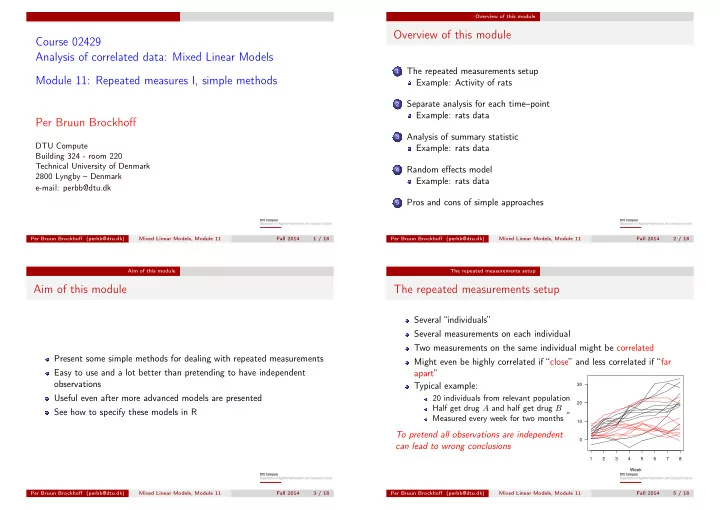
Several “individuals” Several measurements on each individual Two measurements on the same individual might be correlated Might even be highly correlated if “close” and less correlated if “far apart” Typical example:

20 individuals from relevant population Half get drug A and half get drug B Measured every week for two months

To pretend all observations are independent can lead to wrong conclusions

1 2 3 4 5 6 7 8 10 20 30 Week Y

Per Bruun Brockhoff (perbb@dtu.dk) Mixed Linear Models, Module 11 Fall 2014 5 / 18

The repeated measurements setup Example: Activity of rats

Example: Activity of rats

Summary of experiment: 3 treatments: 1, 2, 3 (concentration) 10 cages per treatment 10 contiguous months The response is activity (log(count) of intersections of light beam during 57 hours)

Month log(count) 8.5 9.0 9.5 10.0 10.5 1 2 3 4 5 6 7 8 9 10

Per Bruun Brockhoff (perbb@dtu.dk) Mixed Linear Models, Module 11 Fall 2014 6 / 18 Separate analysis for each time–point

Separate analysis for each time–point

Select a fixed time point The observations at that time (one from each individual) are independent Do a separate analysis for the observations at that time This is not wrong, but (possibly) a lot of information is waisted This can be done for several time–points, but

Difficult to reach a coherent conclusion Sub–tests are not independent Tempting to select time–points that supports out preference Mass significance: If many tests are carried out at 5% level some might be significant by chance. (Bonferroni correction: Use significance level 0.05/n instead of 0.05)

Per Bruun Brockhoff (perbb@dtu.dk) Mixed Linear Models, Module 11 Fall 2014 8 / 18 Separate analysis for each time–point Example: rats data

Separate analysis of rats data

The model at each time–step is: lnci = µ + α(treatmi) + εi , εi ∼ i.i.d. N(0, σ2), i = 1 . . . 30 The result of the ten tests for no treatment effect:

Month 1 2 3 4 5 6 7 8 9 10 F–value 1.22 0.27 1.02 2.30 3.87 4.10 4.70 7.29 4.09 0.88

Compare with F95%;2,27 = 3.35 or F99.5%;2,27 = 6.49 if Bonferroni correction is used

Per Bruun Brockhoff (perbb@dtu.dk) Mixed Linear Models, Module 11 Fall 2014 9 / 18 Analysis of summary statistic

Analysis of summary statistic

Choose a single measure to summarize the individual curves This again reduces the data set to independent observations Popular choices of summary measures:

Average over time Slope in regression with time (or higher order polynomial coefficients) Total increase (last point minus first point) Area under curve (AUC) Maximum or minimum point

Good method with few and easily checked assumptions Information may be lost Important to choose a good summary measure

Per Bruun Brockhoff (perbb@dtu.dk) Mixed Linear Models, Module 11 Fall 2014 11 / 18

Analysis of summary statistic Example: rats data

Rats data analyzed via summary measure

The log of the total activity is chosen as summary measure lnTot = log(Total count) The one way ANOVA model becomes: lnToti = µ + α(treatmi) + εi, εi ∼ i.i.d. N(0, σ2), i = 1 . . . 30 The P–value for no treatment effect in this summary model is 5.23% Notice the simplicity of the model and the relative few assumptions

Per Bruun Brockhoff (perbb@dtu.dk) Mixed Linear Models, Module 11 Fall 2014 12 / 18 Random effects model

Random effects model

This model uses all observations instead of reducing to one

• bservation per individual

Add “individual” as a random effect Makes measurements on same individual correlated Unfortunately equally correlated no matter if they are “close” or “far apart” Can be considered first step in modeling the actual covariance structure Usually only good for short series This model is also known as the split–plot model for repeated measurements (with “individuals” as main–plots and the single measurements as sub–plots)

Per Bruun Brockhoff (perbb@dtu.dk) Mixed Linear Models, Module 11 Fall 2014 14 / 18 Random effects model Example: rats data

Rats data analyzed via random effects approach

The model can now be enhanced to: lnci = µ+α(treatmi)+β(monthi)+γ(treatmi, monthi)+d(cagei)+εi , The covariance structure of this model is: cov(yi1, yi2) =    , if cagei1 = cagei2 and i1 = i2 σ2

d

, if cagei1 = cagei2 and i1 = i2 σ2

d + σ2

, if i1 = i2 A split-plot structure:

treatm is whole plot factor month is sub plot factor

The P–value for the interaction term is 0.0059. Significant, but is the model too simple?

Per Bruun Brockhoff (perbb@dtu.dk) Mixed Linear Models, Module 11 Fall 2014 15 / 18 Pros and cons of simple approaches

Pros and cons of simple approaches

Separate analysis for each time–point + Not wrong – Can be confusing – Difficult to reach coherent conclusion – In general not very informative Analysis of summary statistic + Good method with few and easily checked assumptions – Important to choose good summary measure(s) Random effects approach + Good method for short series + Uses all observations – Usually not good for long series

Per Bruun Brockhoff (perbb@dtu.dk) Mixed Linear Models, Module 11 Fall 2014 17 / 18

Pros and cons of simple approaches

Overview of this module

1

The repeated measurements setup Example: Activity of rats

2

Separate analysis for each time–point Example: rats data

3

Analysis of summary statistic Example: rats data

4

Random effects model Example: rats data

5

Pros and cons of simple approaches

Per Bruun Brockhoff (perbb@dtu.dk) Mixed Linear Models, Module 11 Fall 2014 18 / 18