Overview of this module Course 02429 Analysis of correlated data: - - PowerPoint PPT Presentation

Course 02429 Analysis of correlated data: Mixed Linear Models Module 8: Analysis of covariance Per Bruun Brockhoff

DTU Compute Building 324 - room 220 Technical University of Denmark 2800 Lyngby – Denmark e-mail: perbb@dtu.dk

Per Bruun Brockhoff (perbb@dtu.dk) Mixed Linear Models, Module 8 Fall 2014 1 / 19

Overview of this module

1

The analysis of covariance models Example: Hormone treatment of steers General analysis approach

2

Example with different slopes Analysis of covariance model structures

3

Analysis of covariance in perspective

Per Bruun Brockhoff (perbb@dtu.dk) Mixed Linear Models, Module 8 Fall 2014 2 / 19 The analysis of covariance models Example: Hormone treatment of steers

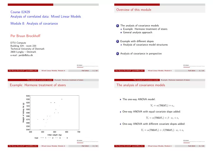
Example: Hormone treatment of steers

Per Bruun Brockhoff (perbb@dtu.dk) Mixed Linear Models, Module 8 Fall 2014 4 / 19 The analysis of covariance models Example: Hormone treatment of steers

The analysis of covariance models

The one-way ANOVA model: Yi = α(TREATi) + ǫi, One-way ANOVA with equal covariate slope added: Yi = α(TREATi) + β · xi + ǫi One-way ANOVA with different covariate slopes added: Yi = α(TREATi) + β(TREATi) · xi + ǫi

Per Bruun Brockhoff (perbb@dtu.dk) Mixed Linear Models, Module 8 Fall 2014 5 / 19

The analysis of covariance models General analysis approach

General analysis approach

1 Test equal slopes model versus different slopes model (Interaction) 2 If significant interaction:

YES, there is a significant treatment effect! Summarize information within the different slopes setting.

3 If NOT significant interaction:

Test the treatment effect in the equal slopes model. (Remove the covariate again if not significant) Summarize information within the equal slopes setting.

Per Bruun Brockhoff (perbb@dtu.dk) Mixed Linear Models, Module 8 Fall 2014 6 / 19 The analysis of covariance models General analysis approach

Example: Hormone treatment of steers.

Randomized Block experiment:

Hormone treatment 1 2 3 4 Weight Y Weight Y Weight Y Weight Y Block 1 560 1330 440 1280 530 1290 690 1340 Block 2 470 1320 440 1270 510 1300 420 1250 Block 3 410 1270 360 1270 380 1240 430 1260 Block 4 500 1320 460 1280 500 1290 540 1310

Different slopes model: Yi = d(BLOCKi) + α(HORMONEi) + β(HORMONEi) · WEIGHTi + ǫi Equal slopes model: Yi = d(BLOCKi) + α(HORMONEi) + β · WEIGHTi + ǫi

Per Bruun Brockhoff (perbb@dtu.dk) Mixed Linear Models, Module 8 Fall 2014 7 / 19 The analysis of covariance models General analysis approach

Steers example: Results

Source of Numerator Denominator F P-value variation degrees degrees

• f freedom
• f freedom

weight 1 3.69 (28.09) (0.0076) treat 3 6.5 (1.59) (0.2821) weight*treat 3 6.61 1.44 0.3147 Source of Numerator degrees Denominator degrees F P variation

• f freedom
• f freedom

weight 1 11 67.5 <0.0001 treat 3 11 6.38 0.0092

Per Bruun Brockhoff (perbb@dtu.dk) Mixed Linear Models, Module 8 Fall 2014 8 / 19 The analysis of covariance models General analysis approach

An analysis ignoring the covariate.

Randomized Block model: Yi = d(BLOCKi) + α(HORMONEi) + ǫi Results:

Source of Numerator degrees Denominator degrees F P variation

• f freedom
• f freedom

treat 3 9 2.04 0.1786

The treatment difference is NOT detected!

Per Bruun Brockhoff (perbb@dtu.dk) Mixed Linear Models, Module 8 Fall 2014 9 / 19

The analysis of covariance models General analysis approach

Summary and post hoc analysis.

The final equal slopes model: Yi = d(BLOCKi) + α(HORMONEi) + β · WEIGHTi + ǫi where d(BLOCKi) ∼ N(0, σ2

B), ǫi ∼ N(0, σ2)

ˆ σ2

B = 0, ˆ

σ2 = 126.1

Parameter Estimate Hormone 1 α(1) 1150.6 Hormone 2 α(2) 1135.3 Hormone 3 α(3) 1122.2 Hormone 4 α(4) 1119.1 Slope β 0.3287

Per Bruun Brockhoff (perbb@dtu.dk) Mixed Linear Models, Module 8 Fall 2014 10 / 19 The analysis of covariance models General analysis approach

Summary and post hoc analysis, cont.

Better with LSMEANS: ˆ α(HORMONEi) + ˆ β · WEIGHT Parameter LSMEAN LOWER UPPER Hormone 1 α(1) + β · 477.5 1308 1295 1320 Hormone 2 α(2) + β · 477.5 1292 1279 1305 Hormone 3 α(3) + β · 477.5 1279 1267 1292 Hormone 4 α(4) + β · 477.5 1276 1263 1289

Per Bruun Brockhoff (perbb@dtu.dk) Mixed Linear Models, Module 8 Fall 2014 11 / 19 Example with different slopes

Example with different slopes

1 1 1 1 1 1 10 15 20 25 30 35 40 30 35 40 x y 2 2 2 2 2 2 3 3 3 3 3 3 4 4 4 4 4 4

Source of Numerator degrees Denominator degrees F P-value variation

• f freedom
• f freedom

X*treat 3 9.34 5.12 0.0233

Per Bruun Brockhoff (perbb@dtu.dk) Mixed Linear Models, Module 8 Fall 2014 13 / 19 Example with different slopes

Summary and post hoc analysis

ˆ σ2

B = 18.25, ˆ

σ2 = 1.20 The regression parameters: Parameter Estimate Treat 1 α(1) 26.8 Treat 2 α(2) 21.9 Treat 3 α(3) 28.6 Treat 4 α(4) 22.4 Slope 1 β(1) 0.219 Slope 2 β(2) 0.496 Slope 3 β(3) 0.263 Slope 4 β(4) 0.443 Tell the story for different values of the covariate: ˆ EYi = ˆ α(k) + ˆ β(k) · x0 Choose Small, medium and large x0 value!

Per Bruun Brockhoff (perbb@dtu.dk) Mixed Linear Models, Module 8 Fall 2014 14 / 19

Example with different slopes Analysis of covariance model structures

Analysis of covariance model structures

2 4 6 8 10 2 3 4 5 6 7 Equal slopes model x y α

1

+ βx α

2

+ βx α

3

+ βx Treat 1 Treat 2 Treat 3 x xLOW xHIGH

• 2

4 6 8 10 1 2 3 4 5 Different slopes model x y α

1

+ β

1

x α2 + β2x α

3

+ β

3

x x xLOW xHIGH

• Per Bruun Brockhoff (perbb@dtu.dk)

Mixed Linear Models, Module 8 Fall 2014 15 / 19 Example with different slopes Analysis of covariance model structures

Summary and post hoc analysis, cont.

1 1 1 1 1 1 10 15 20 25 30 35 40 30 35 40 x y 2 2 2 2 2 2 3 3 3 3 3 3 4 4 4 4 4 4

Per Bruun Brockhoff (perbb@dtu.dk) Mixed Linear Models, Module 8 Fall 2014 16 / 19 Analysis of covariance in perspective

Analysis of covariance in perspective

Covariate measurements

can occur in any type of experiment (Split-plot etc.) can be on different levels (observational unit and/or other factors) can occur on several variables

The general approach:

1

Add the covariate term to the model including interactions.

2

Simplify the interactions with the covariate as much as possible

3

Do the testing, summary and post hoc analysis in the resulting model.

4

If more than one: find the best(s)!

Baseline measurements: ANCOVA better than analyzing differences!

Per Bruun Brockhoff (perbb@dtu.dk) Mixed Linear Models, Module 8 Fall 2014 18 / 19 Analysis of covariance in perspective

Overview of this module

1

The analysis of covariance models Example: Hormone treatment of steers General analysis approach

2

Example with different slopes Analysis of covariance model structures

3

Analysis of covariance in perspective

Per Bruun Brockhoff (perbb@dtu.dk) Mixed Linear Models, Module 8 Fall 2014 19 / 19