Overview of this module Course 02429 Analysis of correlated data: - - PowerPoint PPT Presentation

SLIDE 1

Course 02429 Analysis of correlated data: Mixed Linear Models Module 5: Hierarchical random effects Per Bruun Brockhoff

DTU Compute Building 324 - room 220 Technical University of Denmark 2800 Lyngby – Denmark e-mail: perbb@dtu.dk

Per Bruun Brockhoff (perbb@dtu.dk) Mixed Linear Models, Module 5 Fall 2014 1 / 24

Overview of this module

1

Main example: Lactase in piglets The hierarchial structure

2

One layer model

3

Type I and Type III tests - again

4

Two layer model

5

Three or more layers

6

Comparing different variance structures

7

Alternative confidence limits - balanced situations

Per Bruun Brockhoff (perbb@dtu.dk) Mixed Linear Models, Module 5 Fall 2014 2 / 24

Aim of this module

Present example where hierarchial error structure is natural Introduce one, two, three,. . . layer models Investigate the covariance structure See how to specify such structures in R

Per Bruun Brockhoff (perbb@dtu.dk) Mixed Linear Models, Module 5 Fall 2014 3 / 24 Main example: Lactase in piglets

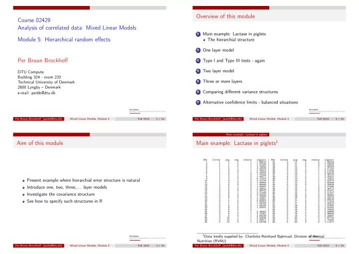
Main example: Lactase in piglets1

Obs litter pig reg status loglact Obs litter pig reg status loglact 1 1 1 1 1 1.89537 31 3 11 1 2 1.58104 2 1 1 2 1 1.97046 32 3 11 2 2 1.52606 3 1 1 3 1 1.78255 33 3 11 3 2 1.65058 4 1 2 1 1 2.24496 34 4 12 1 1 1.97162 5 1 2 2 1 1.43413 35 4 12 2 1 2.11342 6 1 2 3 1 2.16905 36 4 12 3 1 2.51278 7 1 3 1 2 1.74222 37 4 13 1 1 2.06739 8 1 3 2 2 1.84277 38 4 13 2 1 2.25631 9 1 3 3 2 0.17479 39 4 13 3 1 1.79251 10 1 4 1 2 2.12704 40 5 14 1 1 1.93274 11 1 4 2 2 1.90954 41 5 14 2 1 1.82394 12 1 4 3 2 1.49492 42 5 14 3 1 1.23629 13 2 5 1 2 1.62897 43 5 15 1 2 2.07386 14 2 5 2 2 2.26642 44 5 15 2 2 1.96713 15 2 5 3 2 1.96763 45 5 15 3 2 0.47971 16 2 6 1 2 2.01948 46 5 16 1 2 2.01307 17 2 6 2 2 2.56443 47 5 16 2 2 1.85483 18 2 6 3 2 1.16387 48 5 16 3 2 2.18274 19 2 7 1 2 2.20681 49 5 17 1 2 2.86629 20 2 7 2 2 2.55652 50 5 17 2 2 2.71414 21 2 7 3 2 1.69358 51 5 17 3 2 1.60533 22 2 8 1 2 1.09186 52 5 18 1 2 1.97865 23 2 8 2 2 1.93091 53 5 18 2 2 1.93342 24 2 8 3 2 . 54 5 18 3 2 0.74943 25 3 9 1 1 2.36462 55 5 19 1 2 2.89886 26 3 9 2 1 2.72261 56 5 19 2 2 2.88606 27 3 9 3 1 2.80336 57 5 19 3 2 2.20697 28 3 10 1 1 2.42834 58 5 20 1 2 1.87733 29 3 10 2 1 2.64971 59 5 20 2 2 1.70260 30 3 10 3 1 2.54788 60 5 20 3 2 1.11077 1Data kindly supplied by: Charlotte Reinhard Bjørnvad, Division of Animal

Nutrition (RVAU)

Per Bruun Brockhoff (perbb@dtu.dk) Mixed Linear Models, Module 5 Fall 2014 5 / 24

SLIDE 2

Main example: Lactase in piglets The hierarchial structure

The hierarchial structure of the lactase data set

Litter=1 Litter=2 Pig=1 Pig=2 Pig=3 Pig=4 Pig=5 Pig=6 Pig=7 Pig=8 1 2 3 4 5 6 7 8 9 10 11 12 13 14 15 16 17 18 19 20 21 22 23 .

The first layer (counting from the bottom) is the individual measurements i = 1 . . . N. The second layer is the pigs

Pigs could be different, and the model should allow for this If pigs are different, then two measurements on the same pig would be more similar than two from different pigs

The third layer is litters

If litters are different two measurements from the same litter, but different pigs should be correlated, but maybe not as correlated as two from the same pig

(Imagine we had information about farm, area,. . .)

Per Bruun Brockhoff (perbb@dtu.dk) Mixed Linear Models, Module 5 Fall 2014 6 / 24 One layer model

One layer model

The simplest hierarchial model: yi = µ + εi, εi ∼ i.i.d. N(0, σ2) The mean value parameter(s) are estimated by: ˆ β = (X′X)−1X′y The single variance parameter is estimated by: ˆ σ2 = 1 N − p

N

• i=1

(yi − ˆ µi)2 Here is p the number of mean value parameters, and ˆ µi = Xˆ β

Per Bruun Brockhoff (perbb@dtu.dk) Mixed Linear Models, Module 5 Fall 2014 8 / 24 One layer model

Lactase data with one layer model

Consider again the lactase data set, but ignore information about pig and litter A relevant one layer model could be: yi = µ + α(statusi) + β(regi) + γ(statusi, regi) + εi, εi ∼ i.i.d. N(0, σ2) To specify this model in R, we write:

model1 <- lm(loglact ~ reg + status + reg:status, data = lactase) anova(model1)

Part of the R output is:

Analysis of Variance Table Response: loglact Df Sum Sq Mean Sq F value Pr(>F) reg 2 2.5843 1.29217 5.2595 0.008248 ** status 1 1.1288 1.12882 4.5946 0.036680 * reg:status 2 1.4074 0.70368 2.8642 0.065894 . Residuals 53 13.0212 0.24568

• Signif. codes:

0 ‘***’ 0.001 ‘**’ 0.01 ‘*’ 0.05 ‘.’ 0.1 ‘ ’ 1

[I]53

59

status × reg2

6

reg2

3

status1

2

01

1 Per Bruun Brockhoff (perbb@dtu.dk) Mixed Linear Models, Module 5 Fall 2014 9 / 24 Type I and Type III tests - again

Type I (in anova):

Succesive tests Each term is corrected for the terms PREVIOUSLY listed in the model Sums of squares sum to TOTAL sums of squares Depends on the order they are specified in the model

Type III (in drop1 and anova of lmerTest):

Parallel tests Each term is corrected for ALL other the terms in the model Sums of squares do NOT generally sum to TOTAL sums of squares Does NOT depend on the order they are specified in the model

If balanced data: the SAME! drop1 is really ”Type II” = Type III with the condition:

Do NOT test main effects which are part of (fixed) interactions!

Per Bruun Brockhoff (perbb@dtu.dk) Mixed Linear Models, Module 5 Fall 2014 11 / 24

SLIDE 3

Two layer model

Two layer model

The simplest real hierarchial model: yi = µ + a(subi) + εi where a(subi) ∼ N(0, σ2

a), and εi ∼ N(0, σ2), and all (both a’s and

ε’s) are independent The covariance structure is: cov(yi1, yi2) = , if subi1 = subi2 and i1 = i2 σ2

a

, if subi1 = subi2 and i1 = i2 σ2

a + σ2

, if i1 = i2 Or the same expressed via the covariance matrix: V =        σ2

a + σ2

σ2

a

σ2

a

σ2

a

σ2

a + σ2

σ2

a

σ2

a

σ2

a

σ2

a + σ2

σ2

a + σ2

σ2

a

σ2

a

σ2

a

σ2

a + σ2

σ2

a

σ2

a

σ2

a

σ2

a + σ2

      

Per Bruun Brockhoff (perbb@dtu.dk) Mixed Linear Models, Module 5 Fall 2014 13 / 24 Two layer model

Lactase data with two layer model

Now we can include the information about pig: yi = µ + α(statusi) + β(regi) + γ(statusi, regi) + d(pigi) + εi, where d(pigi) ∼ N(0, σ2

d), εi ∼ N(0, σ2), and all independent.

The R code for this model is:

model2 <-model2 <- lmer(loglact ~ reg*status + (1|pig), data = lactase) anova(model2) summary(model2)

Part of the R output is:

Analysis of Variance Table of type 3 with Satterthwaite approximation for degrees of freedom Sum Sq Mean Sq NumDF DenDF F.value Pr(>F) reg 2.77714 1.38857 2 34.921 6.0872 0.005395 ** status 0.34398 0.34398 1 17.683 2.6514 0.121144 reg:status 1.51820 0.75910 2 34.921 5.6265 0.007618 ** [I] status × reg [pig] reg status

Per Bruun Brockhoff (perbb@dtu.dk) Mixed Linear Models, Module 5 Fall 2014 14 / 24 Two layer model

Lactase data with two layer model

More of the of the R (from summary) output is:

Linear mixed model fit by REML ['merModLmerTest'] Formula: loglact ~ reg * status + (1 | pig) Data: lactase REML criterion at convergence: 79.9 Random effects: Groups Name Variance Std.Dev. pig (Intercept) 0.1119 0.3345 Residual 0.1349 0.3673 Fixed effects:Estimate Std. Error df t value Pr(>|t|) (Intercept) 2.129291 0.187780 37.620000 11.339 1.07e-13 *** reg2 0.009363 0.196334 34.810000 0.048 0.9622 reg3

• 0.008660

0.196334 34.810000

• 0.044

0.9651 status2

• 0.121178

0.232912 37.620000

• 0.520

0.6059 reg2:status2 0.109818 0.243523 34.810000 0.451 0.6548 reg3:status2 -0.655019 0.245841 34.980000

• 2.664

0.0116 *

Per Bruun Brockhoff (perbb@dtu.dk) Mixed Linear Models, Module 5 Fall 2014 15 / 24 Three or more layers

Three or more layers

The Basic three layer model is denoted: yi = µ + a(blocki) + b(subi) + εi Here a(blocki) ∼ N(0, σ2

a), b(subi) ∼ N(0, σ2 b), and εi ∼ N(0, σ2)

all independent. The interpretation of the variance parameters: σ2 is the variance between observations from the same subject σ2

b is the variance between subjects within the same block

σ2

a is the variance between blocks

The covariance structure: cov(yi1, yi2) =      , if blocki1 = blocki2 σ2

a

, if blocki1 = blocki2 and subi1 = subi2 σ2

a + σ2 b

, if subi1 = subi2 and i1 = i2 σ2

a + σ2 b + σ2

, if i1 = i2

Per Bruun Brockhoff (perbb@dtu.dk) Mixed Linear Models, Module 5 Fall 2014 17 / 24

SLIDE 4

Three or more layers

Lactase data with three layer model

The model with both litter and pig included: yi = µ + α(statusi) + β(regi) + γ(statusi, regi) +d(litteri) + e(pigi) + εi, where d(litteri) ∼ N(0, σ2

d), e(pigi) ∼ N(0, σ2 e), εi ∼ N(0, σ2)

The R code for this model is:

model3 <- lmer(loglact ~ reg*status + (1|pig) + (1|litter), data = lactase) anova(model3) summary(model3) confint(model3)

Part of the R output is:

Analysis of Variance Table of type 3 with Satterthwaite approximation for degrees of freedom Sum Sq Mean Sq NumDF DenDF F.value Pr(>F) reg 2.77714 1.38857 2 34.921 6.0872 0.005395 ** status 0.34398 0.34398 1 17.683 2.6514 0.121144 reg:status 1.51820 0.75910 2 34.921 5.6265 0.007618 **

[I] status × reg [pig] reg status [litter]

Per Bruun Brockhoff (perbb@dtu.dk) Mixed Linear Models, Module 5 Fall 2014 18 / 24 Three or more layers

Lactase data with three layer model

More R output is:

Linear mixed model fit by REML ['merModLmerTest'] Formula: loglact ~ reg * status + (1 | pig) + (1 | litter) Data: lactase REML criterion at convergence: 79.9 Random effects: Groups Name Variance Std.Dev. pig (Intercept) 0.1119 0.3345 litter (Intercept) 0.0000 0.0000 Residual 0.1349 0.3673 2.5 % 97.5 % .sig01 0.1850922 0.4938041 .sig02 0.0000000 0.2873889 .sigma 0.2829005 0.4426169

Per Bruun Brockhoff (perbb@dtu.dk) Mixed Linear Models, Module 5 Fall 2014 19 / 24 Comparing different variance structures

Comparing different variance structures

Compare two models A and B, where B is a sub–model of A We use the restricted/residual likelihood ratio test:

1

Compute the test value: GA→B = 2ℓ(B)

re − 2ℓ(A) re

2

Lookup the P–value in a χ2

d f statistical table, where

d f = dim(A) − dim(B)

For the lactase data

Model 2ℓre G–value df P–value (A) Pig and litter included 79.9 GA→B = 0.0 1 PA→B = 1 (B) Only pig included 79.9 GB→C = 9.6 1 PB→C = 0.0019 (C) Independent observations 89.5

WARNING: More correct to use df=0.5!!!!

Per Bruun Brockhoff (perbb@dtu.dk) Mixed Linear Models, Module 5 Fall 2014 21 / 24 Alternative confidence limits - balanced situations

Alternative confidence limits - balanced situations

Confidence limit for a variance in a fixed linear model:(of dimension p) (N − p)ˆ σ2 χ2

0.975;(N−p)

< σ2 < (N − p)ˆ σ2 χ2

0.025;(N−p)

If a component is given by: ˆ σ2

A = K

• k=1

bkMSk 95% confidence band can be obtained by: νˆ σ2

A

χ2

0.975;ν

< σ2

A <

νˆ σ2

A

χ2

0.025;ν

ν = (ˆ σ2

A)2

K

k=1

(bkMSk)

2

fk

This is called Satterthwaite approximation

Per Bruun Brockhoff (perbb@dtu.dk) Mixed Linear Models, Module 5 Fall 2014 23 / 24

SLIDE 5

Alternative confidence limits - balanced situations

Overview of this module

1

Main example: Lactase in piglets The hierarchial structure

2

One layer model

3

Type I and Type III tests - again

4

Two layer model

5

Three or more layers

6

Comparing different variance structures

7

Alternative confidence limits - balanced situations

Per Bruun Brockhoff (perbb@dtu.dk) Mixed Linear Models, Module 5 Fall 2014 24 / 24