Overview of this module Course 02429 Analysis of correlated data: - - PowerPoint PPT Presentation

Course 02429 Analysis of correlated data: Mixed Linear Models Module 7: The analysis of split-plot design data Per Bruun Brockhoff

DTU Compute Building 324 - room 220 Technical University of Denmark 2800 Lyngby – Denmark e-mail: perbb@dtu.dk

Per Bruun Brockhoff (perbb@dtu.dk) Mixed Linear Models, Module 7 Fall 2014 1 / 16

Overview of this module

1

Simple Split-plot designs Example: Tenderness of pork.

2

Split-plot with blocks Example: Split-plot with blocks, Yield of oats

3

Split-plot in perspective

Per Bruun Brockhoff (perbb@dtu.dk) Mixed Linear Models, Module 7 Fall 2014 2 / 16 Simple Split-plot designs

Basic structure

a3 b1 a1 b4 a1 b1 a2 b3 a3 b3 a2 b2 a3 b3 a1 b3 a1 b3 a2 b2 a3 b1 a2 b1 a3 b2 a1 b1 a1 b4 a2 b1 a3 b2 a2 b4 a3 b4 a1 b2 a1 b2 a2 b4 a3 b4 a2 b3 Treatments are given on different levels Treatment effects are more easily found on finer levels For B: Randomized block setting with whole-plots as blocks. For A: Completely randomized design with whole-plots as

• bservational unit.

Per Bruun Brockhoff (perbb@dtu.dk) Mixed Linear Models, Module 7 Fall 2014 4 / 16 Simple Split-plot designs Example: Tenderness of pork.

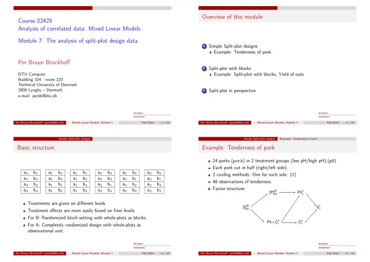
Example: Tenderness of pork.

24 porks (pork) in 2 treatment groups (low pH/high pH).(pH) Each pork cut in half (right/left side). 2 cooling methods: One for each side. (C) 48 observations of tenderness. Factor structure:

[I]22

48

Ph × C1

4

[P]22

24

C1

2

Ph1

2

01

1 Per Bruun Brockhoff (perbb@dtu.dk) Mixed Linear Models, Module 7 Fall 2014 5 / 16

Simple Split-plot designs Example: Tenderness of pork.

The split-plot mixed model for the example

The model: Yi = α(pHi) + β(Ci) + γ(pH × Ci) + d(Pi) + εi pH tested versus the pork (whole plot) variation: F = MSpH MSP C and pH×C tested versus the residual error: F = MSC MSError , F = MSC×pH MSError

Per Bruun Brockhoff (perbb@dtu.dk) Mixed Linear Models, Module 7 Fall 2014 6 / 16 Simple Split-plot designs Example: Tenderness of pork.

Example, test results

Source of Numerator Denominator F P-value variation degrees degrees

• f freedom
• f freedom

phgroup 1 22 8.67 0.0075 cooling 1 22 2.25 0.1479 phgroup*cooling 1 22 0.18 0.6790 Source of Numerator Denominator F P-value variation degrees degrees

• f freedom
• f freedom

phgroup 1 22 8.67 0.0075 cooling 1 22 2.33 0.1403

Per Bruun Brockhoff (perbb@dtu.dk) Mixed Linear Models, Module 7 Fall 2014 7 / 16 Simple Split-plot designs Example: Tenderness of pork.

Example, results summary

Variances: ˆ σ2

W

= 1.2463, ˆ σ2 = 0.4725. Fixed effects: ˆ α(low) = 5.6529, ([4.9240, 6.3819]) ˆ α(high) = 7.1163, ([6.3873, 7.8452])

Per Bruun Brockhoff (perbb@dtu.dk) Mixed Linear Models, Module 7 Fall 2014 8 / 16 Split-plot with blocks Example: Split-plot with blocks, Yield of oats

Example: Split-plot with blocks, Yield of oats

n3 156 n2 118 n2 109 n3 99 v3 n1 140 n0 105 n0 63 n1 70 v3 n0 111 n1 130 n0 80 n2 94 v1 n3 174 n2 157 n3 126 n1 82 v2 n0 117 n1 114 n1 90 n2 100 v2 n2 161 n3 141 n3 116 n0 62 v1 n2 104 n0 70 n3 96 n0 60 v3 n1 89 n3 117 n2 89 n1 102 v2 n3 122 n0 74 n2 112 n3 86 v1 n1 89 n2 81 n0 68 n1 64 v1 n1 103 n0 64 n2 132 n3 124 v2 n2 132 n3 133 n1 129 n0 89 v3 n1 108 n2 126 n2 118 n0 53 v2 n3 149 n0 70 n3 113 n1 74 v1 n3 144 n1 124 n3 104 n2 86 v3 n2 121 n0 96 n0 89 n1 82 v2 n0 61 n3 100 n0 97 n1 99 v1 n1 91 n2 97 n2 119 n3 121 v3

Per Bruun Brockhoff (perbb@dtu.dk) Mixed Linear Models, Module 7 Fall 2014 10 / 16

Split-plot with blocks Example: Split-plot with blocks, Yield of oats

Example: Yield of oats

Factors and their levels: V v1, v2, v3 N n0, n1, n2, n3 P 1, 2, . . . , 18 B 1, 2, . . . , 6 Factor structure:

[I]45

72

V × N6

12

[P]10

18

N3

4

V2

3

[B]5

6

01

1

Per Bruun Brockhoff (perbb@dtu.dk) Mixed Linear Models, Module 7 Fall 2014 11 / 16 Split-plot with blocks Example: Split-plot with blocks, Yield of oats

Yield of oats, exploration

Average yield as a function of nitrogen level for each variety.

Per Bruun Brockhoff (perbb@dtu.dk) Mixed Linear Models, Module 7 Fall 2014 12 / 16 Split-plot with blocks Example: Split-plot with blocks, Yield of oats

Yield of oats, testing

Source of Numerator Denominator F P-value variation degrees degrees

• f freedom
• f freedom

fertil 3 45 37.69 <.0001 variety 2 10 1.49 0.2724 fertil*variety 6 45 0.30 0.9322 Source of Numerator degrees Denominator degrees F P-value variation

• f freedom
• f freedom

fertil 3 51 41.05 <.0001 variety 2 10 1.49 0.2724

Per Bruun Brockhoff (perbb@dtu.dk) Mixed Linear Models, Module 7 Fall 2014 13 / 16 Split-plot in perspective

Split-plot in perspective

Treatments on different levels occur very often in practice More complicated and more than two levels may occur:

Split-plot with correlated whole plots Whole plot conducted as an incomplete latin square A strip-split-split-plot design

The above are case studies in Littel et al. (1999). Serves as a kind of basis for repeated measures analysis.

Per Bruun Brockhoff (perbb@dtu.dk) Mixed Linear Models, Module 7 Fall 2014 15 / 16

Split-plot in perspective

Overview of this module

1

Simple Split-plot designs Example: Tenderness of pork.

2

Split-plot with blocks Example: Split-plot with blocks, Yield of oats

3

Split-plot in perspective

Per Bruun Brockhoff (perbb@dtu.dk) Mixed Linear Models, Module 7 Fall 2014 16 / 16