Constraining fossil fuel CO emissions by the joint assimilation of - - PowerPoint PPT Presentation

▶

Nov 22, 2022 357 likes •552 views

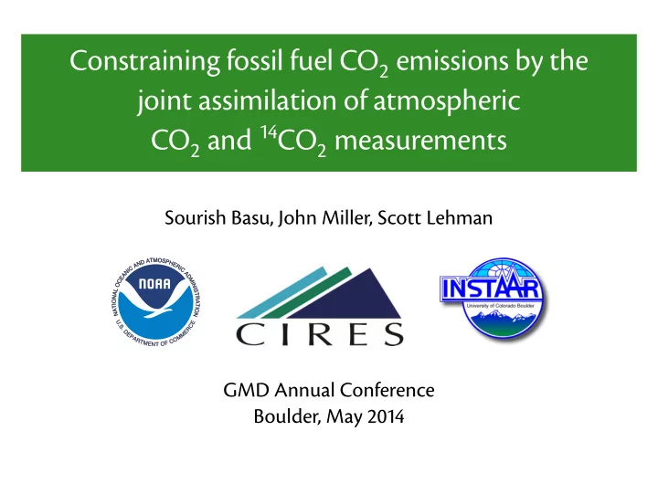
Constraining fossil fuel CO emissions by the joint assimilation of atmospheric CO and CO measurements Sourish Basu, John Miller, Scott Lehman A T M O S P N D H A E R C I I C N A A E D M C O I N L I S

SLIDE 1

Constraining fossil fuel CO emissions by the joint assimilation of atmospheric CO and CO measurements

Sourish Basu, John Miller, Scott Lehman

U . S . D E P A R T M E N T O F C O M M E R C E N A T I O N A L O C E A N I C A N D A T M O S P H E R I C A D M I N I S T R A T I O N

GMD Annual Conference Boulder, May 

SLIDE 2

What is the issue? dC dt = Foce + Fbio + Ffos

0.60 0.45 0.30 0.15 0.00 0.15 0.30 0.45

2010 terrestrial flux

0.0 0.2 0.4 0.6 0.8 1.0 1.2 1.4 1.6 1.8

2010 fossil fuel

◮ Almost all atmospheric CO inversions assume CO(ff) “perfectly”

known, solve for natural fluxes



SLIDE 3

What is the issue? dC dt = Foce + Fbio + Ffos

1.0 0.8 0.6 0.4 0.2 0.0 0.2 0.4 0.6 0.8 1.0

April 2010 terrestrial flux

1.0 0.8 0.6 0.4 0.2 0.0 0.2 0.4 0.6 0.8 1.0

April 2010 fossil fuel spread

◮ Almost all atmospheric CO inversions assume CO(ff) “perfectly”

known, solve for natural fluxes

◮ Only true annually, for global and (some) national totals ◮ Usually not up to date, EDGAR  yr old, Vulcan  yr old



SLIDE 4

CO is a tracer for CO(ff)

∆ Cff = − (i.e., zero CO) Scaling in  = −. ∆ C for  ppm CO(ff) fossil fuel, ocean and land disequilibrium, nuclear and cosmogenic production fossil fuel only



SLIDE 5

NWR CMA

1 2 3 4 5

2010 fossil fuel Miller



SLIDE 6

NWR CMA

1 2 3 4 5

2010 fossil fuel Miller

NWR CMA

1 2 3 4 5

2006 fossil fuel Miller/Vulcan



SLIDE 7

Prior flux uncertainties

◮ US CO(ff): . ±

. Pg CO

◮ Fossil fuel: . ×

inter-prior spread,  km hybrid,  month

◮ Land biosphere: . × respiration per grid cell,  km (e),  month ◮ Ocean:  × abs(net flux),  km (e),  month ◮ Ocean disequilibrium: . × abs(net flux), regional,  month ◮ Land disequilibrium: . × abs(net flux), regional,  month

Our measurements are CO and CO·∆ CO



SLIDE 8

Model-observation mismatch of CO·∆ CO

Mar 2010 Jun 2010 Sep 2010 Dec 2010 Mar 2011 5 10 15 20

CO · ¹ CO mixing ratio

Observations Prior Posterior

Park Falls, Wisconsin, USA (46.0°N, 90.3°W, 472 masl)

Average prior mismatch = . ×  ·ppm Average posterior mismatch = −. ×  ·ppm



SLIDE 9

Model-observation mismatch of CO·∆ CO

Argyle, Maine, USA Boulder Atmospheric Observatory, Colorado, USA Cape May, New jersey, United States Drake Passage Indiana Flux Experiment, USA Park Falls, Wisconsin, USA

Mt. Wilson

Observatory, USA Worcester, Massachusetts, United States Niwot Ridge, Colorado, USA Beech Island, South Carolina, USA Shangdianzi, Peoples Republic of China Tae-ahn Peninsula, Republic of Korea Walnut Grove, California, USA Moody, Texas, USA 4 2 2 4

Residual of CO · ¹ CO AMT BAO CMA DRP INX LEF MWO NHA NWR SCT SDZ TAP WGC WKT

Prior Optimized

Te inversion is doing what it is supposed to do



SLIDE 10

Adjustments to fluxes/optimized emissions

◮ Te CMA–NWR gradient is

consistent with more CO(ff) emission inland

NWR CMA

0.0 0.2 0.4 0.6 0.8 1.0 1.2 1.4 1.6 1.8

2010 fossil fuel Miller



SLIDE 11

Adjustments to fluxes/optimized emissions

◮ Te CMA–NWR gradient is

consistent with more CO(ff) emission inland

◮ Te inversion increases CO(ff)

emission inland

NWR CMA

0.0 0.2 0.4 0.6 0.8 1.0 1.2 1.4 1.6 1.8

2010 fossil fuel Miller

NWR CMA

0.8 0.6 0.4 0.2 0.0 0.2 0.4 0.6 0.8

2010 fossil fuel adjustments



SLIDE 12

Seasonal vs annual CO(ff) adjustments

1.5 1.2 0.9 0.6 0.3 0.0 0.3 0.6 0.9 1.2 1.5

2010 fossil fuel adjustments

◮ Adjustments at the monthly

scale are larger than adjustments at the annual scale

◮ Spatial patterns of the two

adjustments can be different

1.5 1.2 0.9 0.6 0.3 0.0 0.3 0.6 0.9 1.2 1.5

Jan 2010 fossil fuel adjustments

1.5 1.2 0.9 0.6 0.3 0.0 0.3 0.6 0.9 1.2 1.5

Jul 2010 fossil fuel adjustments



SLIDE 13

Points to take home

◮ Fossil fuel CO “well known” at national/yearly scales, not at

regional/monthly scales

◮ Errors in CO(ff) emission estimates cause errors in NEE estimates



SLIDE 14

Points to take home

◮ Fossil fuel CO “well known” at national/yearly scales, not at

regional/monthly scales

◮ Errors in CO(ff) emission estimates cause errors in NEE estimates ◮ CO is a good tracer for CO(ff), can disentangle CO(total) from

CO(ff)

◮ Even with ∼  times lower measurement density, CO

measurements in a CO + CO inversion shifts emission of CO(ff) inland, as expected



SLIDE 15

Points to take home

◮ Fossil fuel CO “well known” at national/yearly scales, not at

regional/monthly scales

◮ Errors in CO(ff) emission estimates cause errors in NEE estimates ◮ CO is a good tracer for CO(ff), can disentangle CO(total) from

CO(ff)

◮ Even with ∼  times lower measurement density, CO

measurements in a CO + CO inversion shifts emission of CO(ff) inland, as expected

◮ Very much a work in progress, not yet the optimal framework for

utilizing CO measurements



SLIDE 16

Mass balance dC dt =Foce + Fbio + Ffos d dt (C · ∆atm) =∆fosFfos + ∆atm (Foce + Fbio) + ∆oceFoce→atm + ∆bioFbio→atm + α (Fnuc + Fcosmo) tracers transported fluxes estimated



SLIDE 17

Uncertainties

◮ US CO(ff): . ± . Pg CO ◮ Land biosphere: . ×

respiration per grid cell,  km (e),  month

◮ Ocean:  × abs(net flux),

 km (e),  month

◮ Fossil fuel: . × inter-prior

spread,  km hybrid,  month

◮ Ocean disequilibrium: . ×

abs(net flux), regional,  month

◮ Land disequilibrium: . ×

abs(net flux), regional,  month



SLIDE 18

Posterior correlation between CO(ff) and CO(nat)

Eastern US Central US Western US Russia G8 China United States Canada Brazil EU27 India 0.4 0.3 0.2 0.1 0.0

Posterior correlation

Traditional No 12C CO2 (FF)

Posterior correlation between CO (nat) and CO (ff) from 01/01/10 to 01/01/11 