
SLIDE 1
Introduction to crystal field multiplet calculations
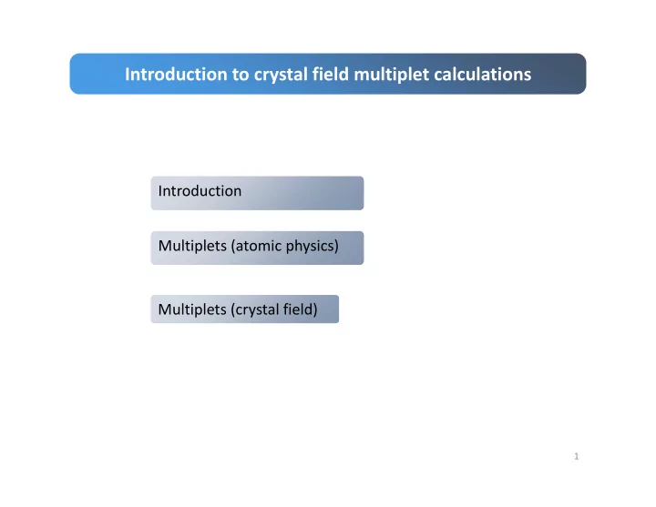
Multiplets (atomic physics) Multiplets (atomic physics) Multiplets (crystal field) Multiplets (crystal field) Introduction Introduction
1
Introduction to crystal field multiplet calculations Introduction - - PowerPoint PPT Presentation
Introduction to crystal field multiplet calculations Introduction Introduction Multiplets (atomic physics) Multiplets (atomic physics) Multiplets (crystal field) Multiplets (crystal field) 1 2p XAS NiO 2p - XAS Experiment is sharper than
1
NiO 2p - XAS L edge
3
L edge
2
L3 edge jump continuum L2 edge jump continuum Intensity (arb. units) 840 845 850 855 860 865 870 875 880 885 Photon energy (eV)
2p
2
3
4
PRB 85, 165113 (2012) PRB 93, 165107 (2016)
5
PRL 107, 107402 (2011).
6
EPL 96, 37007 (2011)
7
core
8
9
10
11
12
13
14
15
16
17
18
+ + k k k k k k J S r e J S
1 2 1 2
12 2
19
+ + k k k k k k J S r e J S
1 2 1 2
12 2
+ + k k k k k k J S r e J S
1 2 1 2
12 2
20
+ + k k k k k k J S r e J S
1 2 1 2
12 2
+ + k k k k k k J S r e J S
1 2 1 2
12 2
21
22
23
24
25
26
1P1, 3P0, 3P1, 3P2 1D2, 3D1, 3D2, 3D3 1F3, 3F2, 3F3, 3F4
27
3 peaks in the spectrum. Why?
28
3 peaks in the spectrum. Why? 3d0→2p53d1 Dipole transition Without spin-orbit coupling Initial state symmetry :
1S
Final state symmetry :
1P, 1D, 1F
Selection rules for dipole transition: ΔL=+1 or -1 ΔS=0 Allowed transition <1S| ∆S=0;∆L=+1 | 1P> ≠0 1 peak in the spectrum
29
3 peaks in the spectrum. Why? 3d0→2p53d1 Dipole transition With spin-orbit coupling Initial state symmetry :
1S0
Final state symmetry :
1P1, 3P0, 3P1, 3P2, 1D2, 3D1, 3D2, 3D3 1F3, 3F2, 3F3, 3F4
Selection rules for dipole transition: ΔJ=+1 or -1 or 0 J=J’≠0 Allowed transitions <1S0|∆J=+1| 1P1, 3P1 , 3D1> ≠0 3 peaks in the spectrum
30
3d0→2p53d1 Dipole transition With spin-orbit coupling Initial state symmetry :
1S0
Final state symmetry :
1P1, 3P0, 3P1, 3P2, 1D2, 3D1, 3D2, 3D3 1F3, 3F2, 3F3, 3F4
Selection rules for dipole transition: ΔJ=+1 or -1 or 0 J=J’≠0 Allowed transitions <1S0|∆J=+1| 1P1, 3P1 , 3D1> ≠0 3 peaks in the spectrum
31
4f0→3d94f1 Dipole transition With spin-orbit coupling Initial state symmetry :
1S0
Final state symmetry :
1P1, 3P0, 3P1, 3P2, 1D2, 3D1, 3D2, 3D3 , 1F3, 3F2, 3F3, 3F4, 1G4, 3G3, 3G4, 3G5, 1H5, 3H4, 3H5, 3H6
Selection rules for dipole transition: ΔJ=+1 or -1 or 0 J=J’≠0 Allowed transitions <1S0|∆J=+1| 1P1, 3P1 , 3D1> ≠0 3 peaks in the spectrum
Calculated Experimental
32
4f0→3d94f1 Dipole transition With spin-orbit coupling Initial state symmetry :
1S0
Final state symmetry :
1P1, 3P0, 3P1, 3P2, 1D2, 3D1, 3D2, 3D3 , 1F3, 3F2, 3F3, 3F4, 1G4, 3G3, 3G4, 3G5, 1H5, 3H4, 3H5, 3H6
Selection rules for dipole transition: ΔJ=+1 or -1 or 0 J=J’≠0 Allowed transitions <1S0|∆J=+1| 1P1, 3P1 , 3D1> ≠0 3 peaks in the spectrum
Calculated Experimental
33
3d0→2p53d1 Dipole transition With spin-orbit coupling (SOC) Selection rules for dipole transition: ΔJ=+1 or -1 or 0 J=J’≠0 Allowed transitions <1S0|∆J=+1| 1P1, 3P1 , 3D1> ≠0 Atomic multiplet theory predicts 3 peaks in the spectrum Calculated Calculated Fk, Gk + SOC
34
3d0→2p53d1 Dipole transition With spin-orbit coupling Selection rules for dipole transition: ΔJ=+1 or -1 or 0 J=J’≠0 Allowed transitions <1S0|∆J=+1| 1P1, 3P1 , 3D1> ≠0 Atomic multiplet theory predicts 3 peaks in the spectrum
Calculated Fk, Gk + SOC
35
36
d orbitals t2g: yz, xz, xy
37
3d0→2p53d1 Dipole transition We need to go beyond the atomic multiplet theory and include the crystal field (CF) in the Hamiltonian
3d0→2p53d1 Dipole transition We need to go beyond the atomic multiplet theory and include the crystal field (CF) in the Hamiltonian
Fk, Gk + SOC + CF eg t2g eg t2g
39
3d6→2p53d7 Dipole transition
775 780 785 790 795 800 805
Energy (eV) Sr2Co0.5Ir0.5O4 Co 2p1/2 Co3+ S=2 Co 2p3/2
775 780 785 790 795 800 805
Co 2p1/2 Co3+ S=0 Energy (eV) NdCaCoO4 Co 2p3/2
40
d orbitals t2g: yz, xz, xy
∆eg>0 ∆t2g>0
b1g: x2-y2 a1g: z2 b2g: xy eg: xz, yz
compressed ∆eg<0 ∆t2g<0
b1g: x2-y2 a1g: z2 b2g: xy eg: xz, yz
41
∆eg=0.48 eV ∆t2g=0.36 eV
b1g: x2-y2 a1g: z2 b2g: xy eg: xz, yz
Ds=0.12 eV, Dt=0 eV
42
43