Shading in OpenGL Shading in OpenGL Polygonal Shading Polygonal - - PDF document

shading in opengl shading in opengl
SMART_READER_LITE
LIVE PREVIEW

Shading in OpenGL Shading in OpenGL Polygonal Shading Polygonal - - PDF document

Shading in OpenGL Shading in OpenGL Polygonal Shading Polygonal Shading Light Source in OpenGL Light Source in OpenGL Material Properties in OpenGL Material Properties in OpenGL Normal Vectors in OpenGL Normal Vectors in OpenGL


slide-1
SLIDE 1

1 Polygonal Shading Light Source in OpenGL Material Properties in OpenGL Normal Vectors in OpenGL Approximating a Sphere [Angel 6.5-6.9] Polygonal Shading Light Source in OpenGL Material Properties in OpenGL Normal Vectors in OpenGL Approximating a Sphere [Angel 6.5-6.9]

Shading in OpenGL Shading in OpenGL

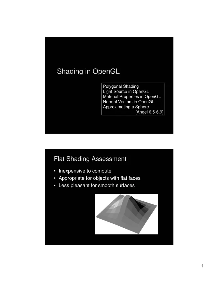
Flat Shading Assessment Flat Shading Assessment

  • Inexpensive to compute
  • Appropriate for objects with flat faces
  • Less pleasant for smooth surfaces
slide-2
SLIDE 2

2

Flat Shading and Perception Flat Shading and Perception

  • Lateral inhibition: exaggerates perceived intensity
  • Mach bands: perceived “stripes” along edges
slide-3
SLIDE 3

3

Interpolative Shading Interpolative Shading

  • Enable with glShadeModel(GL_SMOOTH);
  • Calculate color at each vertex
  • Interpolate color in interior
  • Compute during scan conversion (rasterization)
  • Much better image (see Assignment 1)
  • More expensive to calculate
slide-4
SLIDE 4

4

Gouraud Shading Gouraud Shading

  • Special case of interpolative shading
  • How do we calculate vertex normals?
  • Gouraud: average all adjacent face normals
  • Requires knowledge

about which faces share a vertex—adjacency info

Data Structures for Gouraud Shading Data Structures for Gouraud Shading

  • Sometimes vertex normals can be computed

directly (e.g. height field with uniform mesh)

  • More generally, need data structure for mesh
  • Key: which polygons meet at each vertex
slide-5
SLIDE 5

5

Phong Shading Phong Shading

  • Interpolate normals rather than colors
  • Significantly more expensive
  • Mostly done off-line (not supported in OpenGL)

Phong Shading Results Phong Shading Results

Phong Lighting Gouraud Shading Phong Lighting, Phong Shading Michael Gold, Nvidia

slide-6
SLIDE 6

6

Outline Outline

  • Polygonal Shading
  • Light Sources in OpenGL
  • Material Properties in OpenGL
  • Normal Vectors in OpenGL
  • Example: Approximating a Sphere

Enabling Lighting and Lights Enabling Lighting and Lights

  • Lighting in general must be enabled
  • Each individual light must be enabled
  • OpenGL supports at least 8 light sources

glEnable(GL_LIGHTING); glEnable(GL_LIGHT0);

slide-7
SLIDE 7

7

Global Ambient Light Global Ambient Light

  • Set ambient intensity for entire scene

– The above is default

  • Also: properly light backs of polygons

glLightModeli(GL_LIGHT_MODEL_TWO_SIDED, GL_TRUE)

GLfloat al[] = {0.2, 0.2, 0.2, 1.0}; glLightModelfv(GL_LIGHT_MODEL_AMBIENT, al);

Defining a Light Source Defining a Light Source

  • Use vectors {r, g, b, a} for light properties
  • Beware: light source will be transformed!

GLfloat light_ambient[] = {0.2, 0.2, 0.2, 1.0}; GLfloat light_diffuse[] = {1.0, 1.0, 1.0, 1.0}; GLfloat light_specular[] = {1.0, 1.0, 1.0, 1.0}; GLfloat light_position[] = {-1.0, 1.0, -1.0, 0.0}; glLightfv(GL_LIGHT0, GL_AMBIENT, light_ambient); glLightfv(GL_LIGHT0, GL_DIFFUSE, light_diffuse); glLightfv(GL_LIGHT0, GL_SPECULAR, light_specular); glLightfv(GL_LIGHT0, GL_POSITION, light_position);

slide-8
SLIDE 8

8

Point Source vs Directional Source Point Source vs Directional Source

  • Directional light given by “position” vector
  • Point source given by “position” point

GLfloat light_position[] = {-1.0, 1.0, -1.0, 0.0}; glLightfv(GL_LIGHT0, GL_POSITION, light_position); GLfloat light_position[] = {-1.0, 1.0, -1.0, 1.0}; glLightfv(GL_LIGHT0, GL_POSITION, light_position);

Spotlights Spotlights

  • Create point source as before
  • Specify additional properties to create spotlight

GLfloat sd[] = {-1.0, -1.0, 0.0}; glLightfv(GL_LIGHT0, GL_SPOT_DIRECTION, sd); glLightf (GL_LIGHT0, GL_SPOT_CUTOFF, 45.0); glLightf (GL_LIGHT0, GL_SPOT_EXPONENT, 2.0);

slide-9
SLIDE 9

9

Outline Outline

  • Polygonal Shading
  • Light Sources in OpenGL
  • Material Properties in OpenGL
  • Normal Vectors in OpenGL
  • Example: Approximating a Sphere

Defining Material Properties Defining Material Properties

  • Material properties stay in effect
  • Set both specular coefficients and shininess
  • Diffuse component is analogous

GLfloat mat_a[] = {0.1, 0.5, 0.8, 1.0}; GLfloat mat_d[] = {0.1, 0.5, 0.8, 1.0}; GLfloat mat_s[] = {1.0, 1.0, 1.0, 1.0}; GLfloat low_sh[] = {5.0}; glMaterialfv(GL_FRONT, GL_AMBIENT, mat_a); glMaterialfv(GL_FRONT, GL_DIFFUSE, mat_d); glMaterialfv(GL_FRONT, GL_SPECULAR, mat_s); glMaterialfv(GL_FRONT, GL_SHININESS, low_sh);

slide-10
SLIDE 10

10

Outline Outline

  • Polygonal Shading
  • Light Sources in OpenGL
  • Material Properties in OpenGL
  • Normal Vectors in OpenGL
  • Example: Approximating a Sphere

Defining and Maintaining Normals Defining and Maintaining Normals

  • Define unit normal before each vertex
  • Length changes under some transformations
  • Ask OpenGL to re-normalize (always works)
  • Ask OpenGL to re-scale normal (works for

uniform scaling, rotate, translate)

glNormal3f(nx, ny, nz); glVertex3f(x, y, z); glEnable(GL_NORMALIZE); glEnable(GL_RESCALE_NORMAL);

slide-11
SLIDE 11

11

Example: Icosahedron Example: Icosahedron

  • Define the vertices
  • For simplicity, avoid the use of vertex arrays

#define X .525731112119133606 #define Z .850650808352039932 static GLfloat vdata[12][3] = { {-X, 0, Z}, {X, 0, Z}, {-X, 0, -Z}, {X, 0, -Z}, {0, Z, X}, {0, Z, -X}, {0, -Z, X}, {0, -Z, -X}, {Z, X, 0}, {-Z, X, 0}, {Z, -X, 0}, {-Z, -X, 0} };

Defining the Faces Defining the Faces

  • Index into vertex data array
  • Be careful about orientation!

static GLuint tindices[20][3] = { {1,4,0}, {4,9,0}, {4,9,5}, {8,5,4}, {1,8,4}, {1,10,8}, {10,3,8}, {8,3,5}, {3,2,5}, {3,7,2}, {3,10,7}, {10,6,7}, {6,11,7}, {6,0,11}, {6,1,0}, {10,1,6}, {11,0,9}, {2,11,9}, {5,2,9}, {11,2,7} };

slide-12
SLIDE 12

12

Drawing the Icosahedron Drawing the Icosahedron

  • Normal vector calculation next
  • Should be encapsulated in display list

glBegin(GL_TRIANGLES); for (i = 0; i < 20; i++) { icoNormVec(i); glVertex3fv(&vdata[tindices[i][0]]); glVertex3fv(&vdata[tindices[i][1]]); glVertex3fv(&vdata[tindices[i][2]]); } glEnd();

Calculating the Normal Vectors Calculating the Normal Vectors

  • Normalized cross product of any two sides

GLfloat d1[3], d2[3], n[3]; void icoNormVec (int i) { for (k = 0; k < 3; k++) { d1[k] = vdata[tindices[i][0]] [k] – vdata[tindices[i][1]] [k]; d2[k] = vdata[tindices[i][1]] [k] – vdata[tindices[i][2]] [k]; } normCrossProd(d1, d2, n); glNormal3fv(n); }

slide-13
SLIDE 13

13

The Normalized Cross Product The Normalized Cross Product

  • Omit zero-check for brevity

void normalize(float v[3]) { GLfloat d = sqrt(v[0]*v[0] + v[1]*v[1] + v[2]*v[2]); v[0] /= d; v[1] /= d; v[2] /= d; } void normCrossProd(float u[3], float v[3], float out[3]) {

  • ut[0] = u[1]*v[2] – u[2]*v[1];
  • ut[1] = u[2]*v[0] – u[0]*v[2];
  • ut[2] = u[0]*v[1] – u[1]*v[0];

normalize(out); }

The Icosahedron The Icosahedron

  • Using simple lighting setup
slide-14
SLIDE 14

14

Sphere Normals Sphere Normals

  • Set up instead to use normals of sphere
  • Unit sphere normal is exactly sphere point

glBegin(GL_TRIANGLES); for (i = 0; i < 20; i++) { glNormal3fv(&vdata[tindices[i][0]][0]); glVertex3fv(&vdata[tindices[i][0]][0]); glNormal3fv(&vdata[tindices[i][1]][0]); glVertex3fv(&vdata[tindices[i][1]][0]); glNormal3fv(&vdata[tindices[i][2]][0]); glVertex3fv(&vdata[tindices[i][2]][0]); } glEnd();

Icosahedron with Sphere Normals Icosahedron with Sphere Normals

  • Interpolation vs flat shading effect
slide-15
SLIDE 15

15

Recursive Subdivision Recursive Subdivision

  • General method for building approximations
  • Research topic: construct a good mesh

– Low curvature, fewer mesh points – High curvature, more mesh points – Stop subdivision based on resolution – Some advanced data structures for animation – Interaction with textures

  • Here: simplest case
  • Approximate sphere by subdividing icosahedron

Methods of Subdivision Methods of Subdivision

  • (a) Bisecting angles
  • (b) Computing centroid
  • (c) Bisecting sides
  • Here: bisect sides to retain regularity
slide-16
SLIDE 16

16

Sphere Subdivision: Bisection of Sides Sphere Subdivision: Bisection of Sides

  • Draw if no further subdivision requested

void subdivide(GLfloat v1[3], GLfloat v2[3], GLfloat v3[3], int depth) { GLfloat v12[3], v23[3], v31[3]; int i; if (depth == 0) { drawTriangle(v1, v2, v3); return; } for (i = 0; i < 3; i++) { v12[i] = (v1[i]+v2[i])/2.0; v23[i] = (v2[i]+v3[i])/2.0; v31[i] = (v3[i]+v1[i])/2.0; } ... }

Sphere Subdivision: Extrusion of Midpoints Sphere Subdivision: Extrusion of Midpoints

  • Re-normalize midpoints to lie on unit sphere

void subdivide(GLfloat v1[3], GLfloat v2[3], GLfloat v3[3], int depth) { ... normalize(v12); normalize(v23); normalize(v31); subdivide(v1, v12, v31, depth-1); subdivide(v2, v23, v12, depth-1); subdivide(v3, v31, v23, depth-1); subdivide(v12, v23, v31, depth-1); }

slide-17
SLIDE 17

17

Sphere Subdivision: Start with Icosahedron Sphere Subdivision: Start with Icosahedron

  • In sample code: control depth with ‘+’ and ‘-’

void display(void) { ... for (i = 0; i < 20; i++) { subdivide(&vdata[tindices[i][0]][0], &vdata[tindices[i][1]][0], &vdata[tindices[i][2]][0], depth); } glFlush(); }

Icosahedron Unsubdivided Icosahedron Unsubdivided

slide-18
SLIDE 18

18

One Subdivision One Subdivision Two Subdivisions Two Subdivisions

  • Each time, multiply number of faces by 4
slide-19
SLIDE 19

19

Three Subdivisions Three Subdivisions

  • Reasonable approximation to sphere