SLIDE 1 Shading?
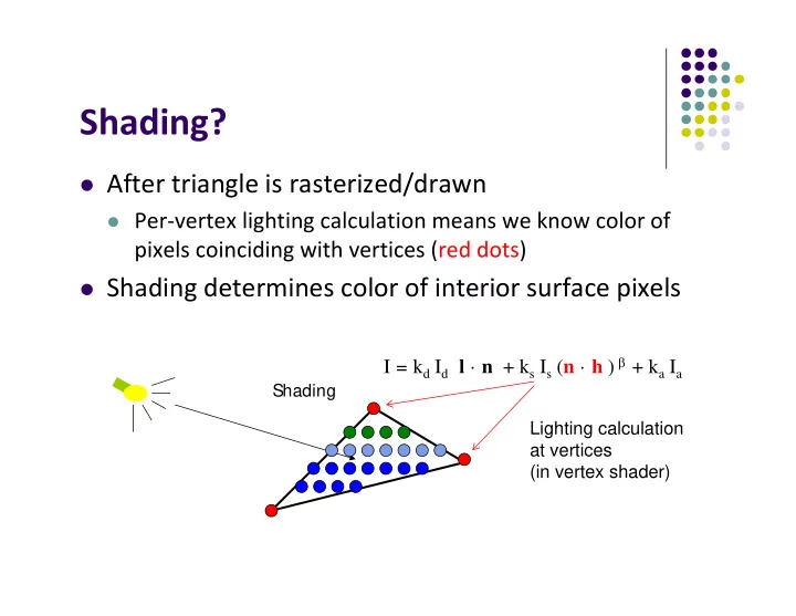
After triangle is rasterized/drawn
Per‐vertex lighting calculation means we know color of
pixels coinciding with vertices (red dots)
Shading determines color of interior surface pixels
Shading
I = kd Id l · n + ks Is (n · h ) + ka Ia
Lighting calculation at vertices (in vertex shader)
SLIDE 2 Shading?
Two types of shading
Assume linear change => interpolate (Smooth shading) No interpolation (Flat shading)
Shading
I = kd Id l · n + ks Is (n · h ) + ka Ia
Lighting calculation at vertices (in vertex shader)
SLIDE 3
Flat Shading
compute lighting once for each face, assign color
to whole face
SLIDE 4 Flat shading
Only use face normal for all vertices in face and
material property to compute color for face
Benefit: Fast! Used when:
Polygon is small enough Light source is far away (why?) Eye is very far away (why?)
Previous OpenGL command: glShadeModel(GL_FLAT)
deprecated!
SLIDE 5 Mach Band Effect
Flat shading suffers from “mach band effect” Mach band effect – human eyes accentuate
the discontinuity at the boundary
Side view of a polygonal surface perceived intensity
SLIDE 6 Smooth shading
Fix mach band effect – remove edge discontinuity Compute lighting for more points on each face 2 popular methods:
Gouraud shading Phong shading Flat shading Smooth shading
SLIDE 7
Gouraud Shading
Lighting calculated for each polygon vertex Colors are interpolated for interior pixels Interpolation? Assume linear change from one vertex
color to another
Gouraud shading (interpolation) is OpenGL default
SLIDE 8
Flat Shading Implementation
Default is smooth shading Colors set in vertex shader interpolated Flat shading? Prevent color interpolation In vertex shader, add keyword flat to output color
flat out vec4 color; //vertex shade …… color = ambient + diffuse + specular; color.a = 1.0;
SLIDE 9
Flat Shading Implementation
Also, in fragment shader, add keyword flat to color
received from vertex shader flat in vec4 color; void main() { gl_FragColor = color; }
SLIDE 10 Gouraud Shading
Compute vertex color in vertex shader Shade interior pixels: vertex color interpolation
C1 C2 C3
Ca = lerp(C1, C2) Cb = lerp(C1, C3)
Lerp(Ca, Cb) for all scanlines * lerp: linear interpolation
SLIDE 11 Linear interpolation Example
If a = 60, b = 40 RGB color at v1 = (0.1, 0.4, 0.2) RGB color at v2 = (0.15, 0.3, 0.5) Red value of v1 = 0.1, red value of v2 = 0.15
a b v1 v2 x
Red value of x = 40 /100 * 0.1 + 60/100 * 0.15 = 0.04 + 0.09 = 0.13 Similar calculations for Green and Blue values
60 40 0.1 0.15 x
SLIDE 12 Gouraud Shading
Interpolate triangle color
1.
Interpolate y distance of end points (green dots) to get color of two end points in scanline (red dots)
2.
Interpolate x distance of two ends of scanline (red dots) to get color of pixel (blue dot)
Interpolate using y values Interpolate using x values
SLIDE 13 Gouraud Shading Function (Pg. 433 of Hill)
for(int y = ybott; y < ytop; y++) // for each scan line { find xleft and xright find colorleft and colorright colorinc = (colorright – colorleft)/ (xright – xleft) for(int x = xleft, c = colorleft; x < xright; x++, c+ = colorinc) { put c into the pixel at (x, y) } } xleft,colorleft xright,colorright ybott ytop
SLIDE 14 Gouraud Shading Implemenation
Vertex lighting interpolated across entire face pixels
if passed to fragment shader in following way
- 1. Vertex shader: Calculate output color in vertex shader,
Declare output vertex color as out
- 2. Fragment shader: Declare color as in, use it, already
interpolated!! I = kd Id l · n + ks Is (n · h ) + ka Ia
SLIDE 15
Calculating Normals for Meshes
For meshes, already know how to calculate face
normals (e.g. Using Newell method)
For polygonal models, Gouraud proposed using
average of normals around a mesh vertex
n = (n1+n2+n3+n4)/ |n1+n2+n3+n4|
SLIDE 16 Gouraud Shading Problem
Assumes linear change across face If polygon mesh surfaces have high curvatures, Gouraud
shading in polygon interior can be inaccurate
Phong shading may look smooth
SLIDE 17 Phong Shading
Need vectors n, l, v, r for all pixels – not provided by user Instead of interpolating vertex color Interpolate vertex normal and vectors Use pixel vertex normal and vectors to calculate Phong
shading at pixel (per pixel lighting)
Phong shading computes lighting in fragment shader
SLIDE 18 Phong Shading (Per Fragment)
Normal interpolation (also interpolate l,v)
n1 n2 n3
nb = lerp(n1, n3) na = lerp(n1, n2) lerp(na, nb)
At each pixel, need to interpolate Normals (n) and vectors v and l
SLIDE 19 Gouraud Vs Phong Shading Comparison
Phong shading more work than Gouraud shading
Move lighting calculation to fragment shaders Just set up vectors (l,n,v,h) in vertex shader
- Set Vectors (l,n,v,h)
- Calculate vertex colors
- Read/set fragment color
- (Already interpolated)
Hardware Interpolates Vertex color
- a. Gouraud Shading
- Set Vectors (l,n,v,h)
- Read in vectors (l,n,v,h)
- (interpolated)
- Calculate fragment lighting
Hardware Interpolates Vectors (l,n,v,h)
I = kd Id l · n + ks Is (n · h ) + ka Ia I = kd Id l · n + ks Is (n · h ) + ka Ia
SLIDE 20 Per‐Fragment Lighting Shaders I
// vertex shader in vec4 vPosition; in vec3 vNormal; // output values that will be interpolatated per-fragment
- ut vec3 fN;
- ut vec3 fE;
- ut vec3 fL;
uniform mat4 ModelView; uniform vec4 LightPosition; uniform mat4 Projection;
Declare variables n, v, l as out in vertex shader
SLIDE 21 void main() { fN = vNormal; fE = -vPosition.xyz; fL = LightPosition.xyz; if( LightPosition.w != 0.0 ) { fL = LightPosition.xyz - vPosition.xyz; } gl_Position = Projection*ModelView*vPosition; }
Per‐Fragment Lighting Shaders II
Set variables n, v, l in vertex shader
SLIDE 22 Per‐Fragment Lighting Shaders III
// fragment shader // per-fragment interpolated values from the vertex shader in vec3 fN; in vec3 fL; in vec3 fE; uniform vec4 AmbientProduct, DiffuseProduct, SpecularProduct; uniform mat4 ModelView; uniform vec4 LightPosition; uniform float Shininess;
Declare vectors n, v, l as in in fragment shader (Hardware interpolates these vectors)
SLIDE 23 Per=Fragment Lighting Shaders IV
void main() { // Normalize the input lighting vectors vec3 N = normalize(fN); vec3 E = normalize(fE); vec3 L = normalize(fL); vec3 H = normalize( L + E ); vec4 ambient = AmbientProduct;
I = kd Id l · n + ks Is (n · h ) + ka Ia
Use interpolated variables n, v, l in fragment shader
SLIDE 24 float Kd = max(dot(L, N), 0.0); vec4 diffuse = Kd*DiffuseProduct; float Ks = pow(max(dot(N, H), 0.0), Shininess); vec4 specular = Ks*SpecularProduct; // discard the specular highlight if the light's behind the vertex if( dot(L, N) < 0.0 ) specular = vec4(0.0, 0.0, 0.0, 1.0); gl_FragColor = ambient + diffuse + specular; gl_FragColor.a = 1.0; }
Per‐Fragment Lighting Shaders V
I = kd Id l · n + ks Is (n · h ) + ka Ia
Use interpolated variables n, v, l in fragment shader
SLIDE 25
Toon (or Cel) Shading
Non‐Photorealistic (NPR) effect Shade in bands of color
SLIDE 26 Toon (or Cel) Shading
How? Consider (l · n) diffuse term (or cos Θ) term Clamp values to min value of ranges to get toon
shading effect I = kd Id l · n + ks Is (n · h ) + ka Ia
l · n Value used Between 0.75 and 1 0.75 Between 0.5 and 0.75 0.5 Between 0.25 and 0.5 0.25 Between 0.0 and 0.25 0.0
SLIDE 27 BRDF Evolution
BRDFs have evolved historically
1970’s: Empirical models
Phong’s illumination model
1980s:
Physically based models
Microfacet models (e.g. Cook Torrance model)
1990’s
Physically‐based appearance models of specific effects (materials, weathering, dust, etc)
Early 2000’s
Measurement & acquisition of static materials/lights (wood, translucence, etc)
Late 2000’s
Measurement & acquisition of time‐varying BRDFs (ripening, etc)
SLIDE 28 Physically‐Based Shading Models
Phong model produces pretty pictures Cons: empirical (fudged?) (cos), plastic look Shaders can implement better lighting/shading models Big trend towards Physically‐based lighting models Physically‐based? Based on physics of how light interacts with actual surface Apply Optics/Physics theories Classic: Cook‐Torrance shading model (TOGS 1982)
SLIDE 29 Cook‐Torrance Shading Model
Same ambient and diffuse terms as Phong New, better specular component than (cos), Idea: surfaces has small V‐shaped microfacets (grooves) Many grooves at each surface point Distribution term D: Grooves facing a direction contribute E.g. half of grooves face 30 degrees, etc
v n DG F
, cos
Incident light Average normal n microfacets δ
SLIDE 30 BV BRDF Viewer
BRDF viewer (View distribution of light bounce)
SLIDE 31 BRDF Evolution
BRDFs have evolved historically
1970’s: Empirical models
Phong’s illumination model
1980s:
Physically based models
Microfacet models (e.g. Cook Torrance model)
1990’s
Physically‐based appearance models of specific effects (materials, weathering, dust, etc)
Early 2000’s
Measurement & acquisition of static materials/lights (wood, translucence, etc)
Late 2000’s
Measurement & acquisition of time‐varying BRDFs (ripening, etc)
SLIDE 32 Measuring BRDFs
Murray‐Coleman and Smith Gonioreflectometer. ( Copied and Modified from [Ward92] ).
SLIDE 33
Measured BRDF Samples
Mitsubishi Electric Research Lab (MERL)
http://www.merl.com/brdf/
Wojciech Matusik MIT PhD Thesis 100 Samples
SLIDE 34 BRDF Evolution
BRDFs have evolved historically
1970’s: Empirical models
Phong’s illumination model
1980s:
Physically based models
Microfacet models (e.g. Cook Torrance model)
1990’s
Physically‐based appearance models of specific effects (materials, weathering, dust, etc)
Early 2000’s
Measurement & acquisition of static materials/lights (wood, translucence, etc)
Late 2000’s
Measurement & acquisition of time‐varying BRDFs (ripening, etc)
SLIDE 35 Time‐varying BRDF
BRDF: How different materials reflect light Time varying?: how reflectance changes over time Examples: weathering, ripening fruits, rust, etc
SLIDE 36
References
Interactive Computer Graphics (6th edition), Angel
and Shreiner
Computer Graphics using OpenGL (3rd edition), Hill
and Kelley