SLIDE 1 Computer Graphics (Fall 2008) Computer Graphics (Fall 2008)
COMS 4160, Lecture 18: Illumination and Shading 1
http://www.cs.columbia.edu/~cs4160
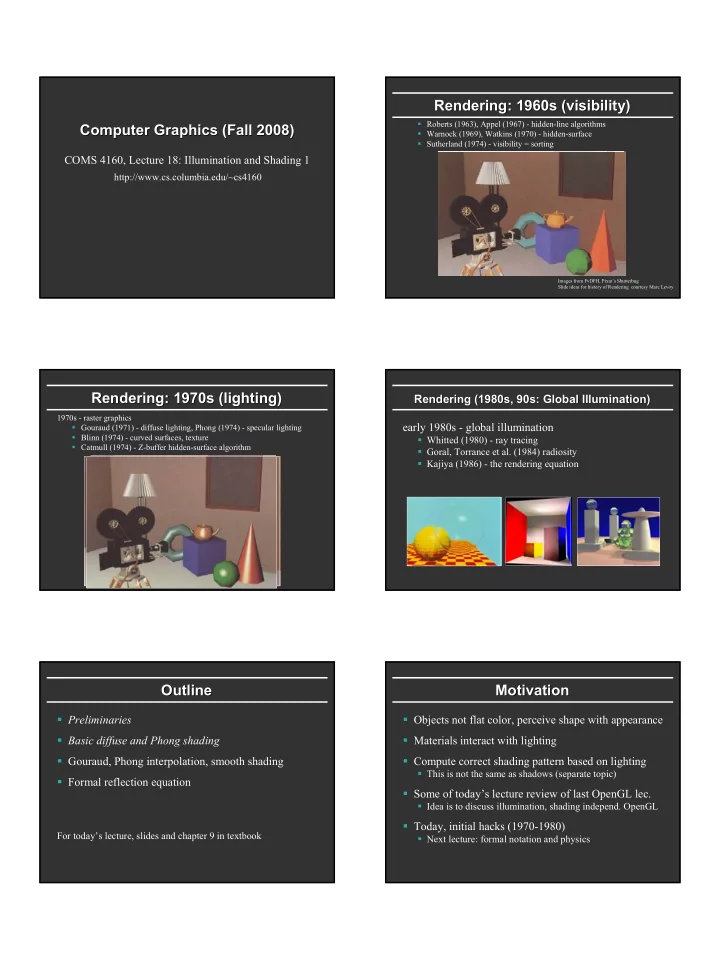
Rendering: 1960s (visibility) Rendering: 1960s (visibility)
Roberts (1963), Appel (1967) - hidden-line algorithms Warnock (1969), Watkins (1970) - hidden-surface Sutherland (1974) - visibility = sorting
Images from FvDFH, Pixar’s Shutterbug Slide ideas for history of Rendering courtesy Marc Levoy
1970s - raster graphics Gouraud (1971) - diffuse lighting, Phong (1974) - specular lighting Blinn (1974) - curved surfaces, texture Catmull (1974) - Z-buffer hidden-surface algorithm
Rendering: 1970s (lighting) Rendering: 1970s (lighting)
Rendering (1980s, 90s: Global Illumination) Rendering (1980s, 90s: Global Illumination) early 1980s - global illumination
Whitted (1980) - ray tracing Goral, Torrance et al. (1984) radiosity Kajiya (1986) - the rendering equation
Outline Outline
Preliminaries Basic diffuse and Phong shading Gouraud, Phong interpolation, smooth shading Formal reflection equation
For today’s lecture, slides and chapter 9 in textbook
Motivation Motivation
Objects not flat color, perceive shape with appearance Materials interact with lighting Compute correct shading pattern based on lighting
This is not the same as shadows (separate topic)
Some of today’s lecture review of last OpenGL lec.
Idea is to discuss illumination, shading independ. OpenGL
Today, initial hacks (1970-1980)
Next lecture: formal notation and physics