
Logistic Regression: MLE vs. OLS3 in Excel2013 25 Aug 2016 V0H 2014-Schield-Logistic-MLE-OLS3-Excel2013-Slides.pdf 1
Schield MLE vs. OLS3-Based Logistic Excel 2013V0H 1
by Milo Schield Member: International Statistical Institute US Rep: International Statistical Literacy Project Director, W. M. Keck Statistical Literacy Project
Slides and data at: www.StatLit.org/
pdf/2014-Schield-Logistic-MLE-OLS3-Excel2013-slides.pdf Excel/2014-Schield-Logistic-MLE-OLS3-Excel2013.xlsx
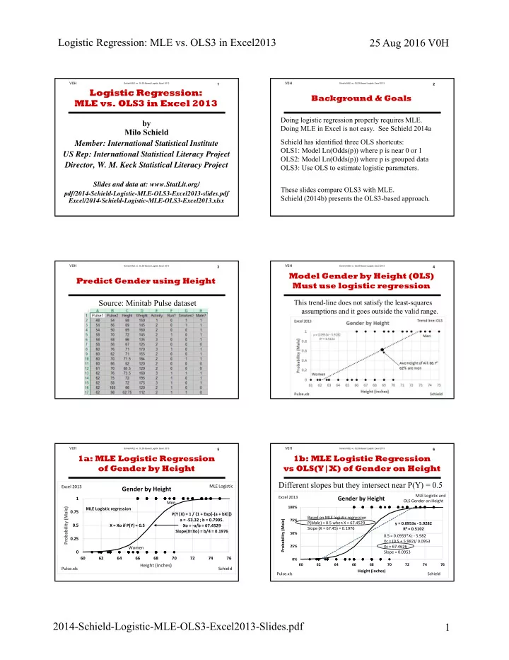
Logistic Regression: MLE vs. OLS3 in Excel 2013
Schield MLE vs. OLS3-Based Logistic Excel 2013V0H 2
Background & Goals
Doing logistic regression properly requires MLE. Doing MLE in Excel is not easy. See Schield 2014a Schield has identified three OLS shortcuts: OLS1: Model Ln(Odds(p)) where p is near 0 or 1 OLS2: Model Ln(Odds(p)) where p is grouped data OLS3: Use OLS to estimate logistic parameters. These slides compare OLS3 with MLE. Schield (2014b) presents the OLS3-based approach.
Schield MLE vs. OLS3-Based Logistic Excel 2013V0H
Source: Minitab Pulse dataset
3
Predict Gender using Height
Schield MLE vs. OLS3-Based Logistic Excel 2013V0H 4
Model Gender by Height (OLS) Must use logistic regression
This trend-line does not satisfy the least-squares assumptions and it goes outside the valid range. but it does pass through the joint mean.
Schield MLE vs. OLS3-Based Logistic Excel 2013V0H 5
1a: MLE Logistic Regression
- f Gender by Height
0.25 0.5 0.75 1 60 62 64 66 68 70 72 74 76 Probability (Male) Height (inches)
Gender by Height
Pulse.xls MLE Logistic Schield Excel 2013 Women Men MLE Logistic regression P(Y|X) = 1 / {1 + Exp[‐(a + bX)]} a = ‐53.32 ; b = 0.7905. Xo = ‐a/b = 67.4529 Slope(X=Xo) = b/4 = 0.1976 X = Xo if P(Y) = 0.5
Schield MLE vs. OLS3-Based Logistic Excel 2013V0H
Different slopes but they intersect near P(Y) = 0.5
6
1b: MLE Logistic Regression vs OLS(Y|X) of Gender on Height
y = 0.0953x ‐ 5.9282 R² = 0.5102
0% 25% 50% 75% 100% 60 62 64 66 68 70 72 74 76
Probability (Male) Height (inches)
Gender by Height
Excel 2013 MLE Logistic and OLS Gender on Height Pulse.xls Schield 0.5 = 0.0953*Xc ‐ 5.982 Xc = (0.5 + 5.982)/ 0.0953 Xc = 67.4626 Slope = 0.0953 Based on MLE logistic regression P(Male) = 0.5 when X = 67.4529 Slope (X = 67.45) = 0.1976