Workshop 10.5a: Logistic regression Murray Logan August 23, 2016 - - PDF document

• 1-

Workshop 10.5a: Logistic regression

Murray Logan

August 23, 2016

Table of contents

1 Logistic regression 1 2 Worked Examples 5

• 1. Logistic regression

1.1. Logistic regression

1.1.1. Binary data Link: log (

π 1−π

) Transform scale of linear predictor (−∞, ∞) into that of the response (0,1)

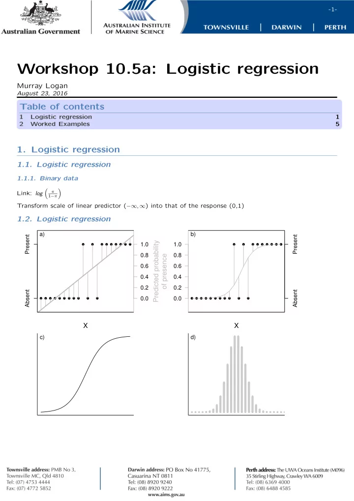
1.2. Logistic regression

• ● ● ● ● ● ● ● ●
• ● ● ● ● ● ●

Absent Present 0.0 0.2 0.4 0.6 0.8 1.0

Predicted probability

• f presence

a)

X

• ● ● ● ● ● ● ● ●
• ● ● ● ● ● ●

Absent Present 0.0 0.2 0.4 0.6 0.8 1.0 b)

X

c) d)

• 2-

1.3. Logistic regression Probability density function

n = 50 n = 20 n = 3 5 10 15 20 25 30 35 40

Cumulative density function

5 10 15 20 25 30 35 40 E(Y ) = ( n x ) px(1 − p)n−x Spread assumed to be equal to mean. (φ = 1)

1.4. Dispersion

1.4.1. Over-dispersion Sample more varied than expected from its mean

• variability due to other unmeasured influences

– quasi- model

• due to more zeros than expected

– zero-inflated model

1.5. Logistic regression

Example data y x 1 0 1.024733 2 0 2.696719 3 0 3.626263 4 0 4.948643 5 0 6.024718 6 0 6.254113

• 3-
• ●
• ●●
• −0.5

0.0 0.5 1.0 1.5 5 10 15

x y

• ●
• ●●
• −0.5

0.0 0.5 1.0 1.5 5 10 15

x y

1.6. Logistic regression

• Fit model

> dat.glmL <- glm(y ~ x, data = dat, family = "binomial")

1.7. Logistic regression

• Explore residuals

> par(mfrow=c(2,2)) > plot(dat.glmL)

−6 −4 −2 2 4 −2 −1 1 2 Predicted values Residuals

• ●
• ●
• Residuals vs Fitted

• −2

−1 1 2 −2 −1 1 2 Theoretical Quantiles

• Std. deviance resid.

Normal Q−Q

−6 −4 −2 2 4 0.0 0.5 1.0 1.5 Predicted values

• Std. deviance resid.
• Scale−Location

0.00 0.05 0.10 0.15 −3 −2 −1 1 2 Leverage

• Std. Pearson resid.
• ● ●
• Cook's distance

Residuals vs Leverage

1.8. Logistic regression

• Explore goodness of fit
• Pearson’s χ2 residuals

> dat.resid <- sum(resid(dat.glmL, type = "pearson")^2) > 1 - pchisq(dat.resid, dat.glmL$df.resid)

[1] 0.8571451

• Deviance (G 2)

• 4-

> 1-pchisq(dat.glmL$deviance, dat.glmL$df.resid)

[1] 0.8647024

1.9. Logistic regression

• Explore model parameters

Slope parameter is on log odds-ratio scale

> summary(dat.glmL)

Call: glm(formula = y ~ x, family = "binomial", data = dat) Deviance Residuals: Min 1Q Median 3Q Max

• 1.97157
• 0.33665
• 0.08191

0.30035 1.59628 Coefficients: Estimate Std. Error z value Pr(>|z|) (Intercept)

• 6.9899

3.1599

• 2.212

0.0270 * x 0.6559 0.2936 2.234 0.0255 *

• Signif. codes:

0 '***' 0.001 '**' 0.01 '*' 0.05 '.' 0.1 ' ' 1 (Dispersion parameter for binomial family taken to be 1) Null deviance: 27.526

• n 19

degrees of freedom Residual deviance: 11.651

• n 18

degrees of freedom AIC: 15.651 Number of Fisher Scoring iterations: 6

1.10. Logistic regression

• Quasi R2

quasiR2 = 1 − ( deviance null deviance )

> 1-(dat.glmL$deviance/dat.glmL$null)

[1] 0.5767057

1.11. Logistic regression

• LD50

LD50 = −intercept slope

> -dat.glmL$coef[1]/dat.glmL$coef[2]

(Intercept) 10.65781

• 5-

1.12. Logistic regression

• summary figure
• ● ●
• 0.00

0.25 0.50 0.75 1.00 5 10 15

x Y

• 2. Worked Examples

• 6-

2.1. Worked Examples

• Algiv./Detritiv.

Invertivore Omnivore Piscivore 0.0 0.2 0.4 0.6 0.8

0.10 −0.4 0.0 0.2 0.4 Residuals

• ●
• ●
• ●
• ●
• ●
• 0.10

0.0 0.5 1.0 1.5 Standardized residuals

• Error in qt(0.975, df = arrington.glm$df.resid): object 'arrington.glm' not found

• 7-
• 0.1

0.2 0.3 Algiv./Detritiv. Invertivore Omnivore Piscivore

Trophic fit

−15 −5 5 10 Residuals

• 5

10 15 20

• Std. deviance resid.