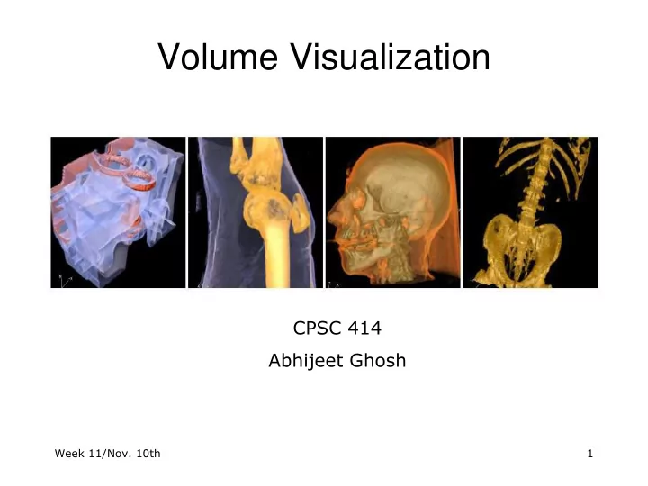
Volume Visualization CPSC 414 Abhijeet Ghosh Week 11/Nov. 10th 1 - - PowerPoint PPT Presentation

Volume Visualization

CPSC 414 Abhijeet Ghosh

Week 11/Nov. 10th 1

Surface Graphics

• Objects explicitly defined by a surface or

boundary representation:

– a mesh of polygons

Week 11/Nov. 10th 2

Surface Graphics

• Pros

– fast rendering algorithms available – hardware acceleration cheap (PC game boards!) – OpenGL API for programming – use texture mapping for added realism

• Cons

– discards interior of object, maintaining only the shell – operations such cutting, slicing & dissection not possible – no artificial viewing modes such as semi-transparencies, X-ray – surface-less phenomena such as clouds, fog & gas are hard to model and represent

Week 11/Nov. 10th 3

Volume Graphics

• Maintains a discrete representation close to

the underlying 3D object

• Different aspects of the dataset can be

emphasized via changes in transfer functions

– translate raw densities into colors and transparencies

• When the nature of the data is not known, it is

difficult to create the right polygonal mesh

– easier to voxelize!

Week 11/Nov. 10th 4

Volume Graphics

• Pros

– formidable technique for data exploration

volumetric human head (CT scan)

• Cons

– rendering algorithm has high complexity! – special purpose hardware costly (~$3,000-$10,000)

Week 11/Nov. 10th 5

Volume Graphics – Examples

Anatomical atlas from visible human (CT & MRI) datasets Industrial CT - structural failure and security applications flow around an airplane wing Shockwave visualization – simulation with Navier-Stokes PDEs

Week 11/Nov. 10th 6

Volume Graphics - Basics

• A volume is 3D array of point samples, called voxels

– the point samples are located at the grid points – the process of generating a 2D image from the 3D volume is called volume rendering

Week 11/Nov. 10th 7

Volume Rendering Pipeline

raw density data (voxel)

Week 11/Nov. 10th 8

classification interpolation shading compositing interpolation classification

Classification

• A raw voxel stores only density
• Density may have a different meanings:

– stress, strain, temperature – absorption – material tag

• Need for assigning meaningful visual attributes such as colors
• Classification is translation of raw values to color and opacity
• Classification done using RGBα transfer functions!

Week 11/Nov. 10th 9

Transfer Functions

1.0 0.0 Voxel density

gel - transparent tissue – semi- transparent bone – opaque

255

Week 11/Nov. 10th 10

Volume Rendering Modes

• For each pixel in the image, a ray is cast

into the volume:

• Four main volume rendering modes exist:

eye

X-Ray:

Rays sum contributions along their path linearly

Maximum Intensity Projection:

A pixel stores the largest intensity values along its ray

Iso-surface:

Rays com posite contributions only from voxels of a certain intensity defining a surface

Full-volume:

Rays com posite contributions along their path linearly Week 11/Nov. 10th 11

Ray casting – Orthographic

All rays are parallel A ray is specified as: rij = n, the view vector n = u × v Image order projection:

• scan the image in row order,

Pi, j = P0, 0 + j(Ni -1) + i

• Pi, j location of pixel i, j in world space

0<=i<=Ni 0<=j<=Nj P0, 0 = image origin in world space A point P on a ray is given by: P = Pi, j + t × n t = step size along ray

Week 11/Nov. 10th 12

Ray casting – Perspective

A ray is specified by:

• eye position (Eye)
• screen pixel location (Pi, j)

rij = the view vector = Pi, j – Eye / | Pi, j – Eye | Image order projection:

• scan the image in row order,

Pi, j = P0, 0 + j(Ni -1) + i

• Pi, j location of pixel i, j in world space

0<=i<=Ni 0<=j<=Nj P0, 0 = image origin in world space A point P on a ray is given by: P = Eye + t × ri, j t = step size along ray

Week 11/Nov. 10th 13

Volume Rendering Integral

• Consider a volume consisting of particles:

– each has color C and light attenuating density µ

• A rendering ray accumulates attenuated colors
• The continuous volume rendering integral:
• Approximate it by discretizing it into sampling intervals of width ∆s:

analytic evaluation of the integral not efficient

Week 11/Nov. 10th 14

Volume Rendering Integral

• A few approximations make the computation more efficient
• Define transparency t(i∆s) as:

exp(-µ(i∆s) ∆s) = t(i∆s)

• Opacity α is defined as (1 - transparency): α(i∆s) = (1 – t(i∆s))
• Approximate the exponential term by a two term Taylor expansion:

t(i∆s) = exp(-µ(i∆s) ∆s) ≈ 1 - µ(i∆s) ∆s

• Then we can write:

µ(i∆s) ∆s ≈ 1 – t(i∆s) = α(i∆s)

• Discretized volume rendering integral:
• This equation is used for stepwise compositing of samples along a ray

Week 11/Nov. 10th 15

Compositing

• It is the accumulation of colors weighted by opacities
• Colors and opacities of back pixels are attenuated by opacities
• f front pixels:

rgb = RGBback αback (1 – αfront) + RGBfront αfront α = αback (1 – αfront ) + αfront

• This leads to the front-to-back compositing equation:

c = C(i∆s)α(i∆s)(1 - α) + c α = α(i∆s)(1 - α) + α

• back-to-front compositing:

c = c(1 - α(i∆s)) + C(i∆s) α = α (1 - α(i∆s)) + α(i∆s)

advantage – early ray termination! advantage – object order approach suitable for hardware implementation!

Week 11/Nov. 10th 16

Volume Rendering Algorithms

• Ray casting

– image order, forward viewing

• Splatting

– object order, backward viewing

• 2D & 3D texture mapping h/w

– object order – back-to-front compositing

Week 11/Nov. 10th 17

Splatting

• Each voxel represented as a fuzzy ball

(a 3D Gaussian function)

• Each such fuzzy voxel is given an RGBα value

– based on the transfer function

• Fuzzy balls projected onto the screen, leaving a footprint called splat
• Simplified algorithm:

– traverse the voxels in front-to-back order – project the voxels to the screen and composite the splats

• bject order algorithm – project
• nly interesting voxels hence fast

Week 11/Nov. 10th 18

Texture Mapping

• 2D: volume as axis aligned 2D textures

– back-to-front compositing – coherent memory access pattern – commodity hardware support – need for calculating texture coordinates and warping to image plane

• 3D: volume as image aligned 3D textures

– requires more complex hardware – current generation PC game boards! – simpler algorithm for generating texture coordinates (directly use u, v, w)

• OpenGL support for compositing

glEnable(GL_BLEND); glBlendFunc(GL_SRC_ALPHA, GL_ONE_MINUS_SRC_ALPHA); Week 11/Nov. 10th 19

Volume Visualization

• Acknowledgement:

Klaus Mueller mueller@cs.sunysb.edu Stony Brook University New York - 11794, USA

Week 11/Nov. 10th 20