5. Volume Visualization Scalar volume data Medical Applications: - PDF document

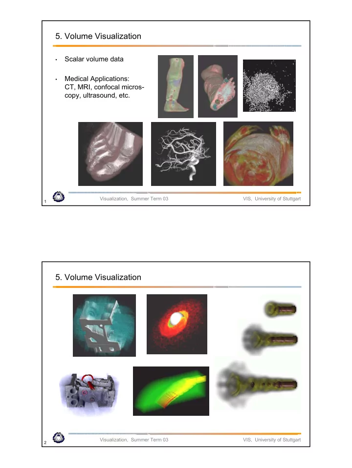
5. Volume Visualization Scalar volume data • Medical Applications: • CT, MRI, confocal micros- copy, ultrasound, etc. Visualization, Summer Term 03 VIS, University of Stuttgart 1 5. Volume Visualization Visualization, Summer Term 03 VIS, University of Stuttgart 2

5. Volume Visualization Visualization, Summer Term 03 VIS, University of Stuttgart 3 5. Volume Visualization Some possible characteristics of volume data • Essential information in the interior • Can not be described by geometric representation • (fire, clouds, gaseous phenomena) Distinguish between shape (given by the geometry of the grid) and appearance • (given by the scalar values) Even if the data could be described geometrically, there are, in general, too many • primitives to be represented Visualization, Summer Term 03 VIS, University of Stuttgart 4

5. Volume Visualization Volume rendering techniques • Techniques for 2D scalar fields • Indirect volume rendering techniques (e.g. surface fitting) • Convert/reduce volume data to an intermediate representation (surface • representation), which can be rendered with traditional techniques Direct volume rendering • Consider the data as a semi-transparent gel with physical properties and directly get a • 3D representation of it Visualization, Summer Term 03 VIS, University of Stuttgart 5 5. Volume Visualization Slicing: Slice • Display the volume data, mapped to colors, on a slice plane Isosurfacing: • Generate opaque/semi-opaque surfaces Transparency effects: • Volume material attenuates reflected or emitted light Semi-transparent Isosurface material Visualization, Summer Term 03 VIS, University of Stuttgart 6

5. Volume Visualization • 2D visualization slice images (MPR) • Indirect 3D visualization isosurfaces (SSD) • Direct 3D visualization volume rendering (DVR) Visualization, Summer Term 03 VIS, University of Stuttgart 7 5. Volume Visualization Direct volume rendering techniques • Direct volume rendering allows for the "global" representation integrating physical • characteristics But prohibits interactive display due to its numerical complexity, in general • Indirect volume rendering techniques • Often result in complex representations • Pre-processing the surface representation might help • Use graphics hardware for interactive display • Goal • Integrate different techniques in order to represent the data as "good" as possible • But, keep in mind that the most correct method in terms of physical realism must • not be the most optimal one in terms of understanding the data Visualization, Summer Term 03 VIS, University of Stuttgart 8

5. Volume Visualization Different grid structures: • Structured: uniform, rectilinear, curvilinear • Unstructured • Scattered data • Visualization, Summer Term 03 VIS, University of Stuttgart 9 5. Volume Visualization Pixel (picture element) • Voxel (volume element) • Values are constant within a region around a grid point • Cell • Values between grid points are resampled by interpolation • Visualization, Summer Term 03 VIS, University of Stuttgart 10

5.1. Classification Color table for volume visualization • Maps raw voxel value into presentable entities: • color, intensity, opacity, etc. Transfer function • Goals and issues: • Empowers user to select “structures” • Extract important features of the data set • Classification is non trivial • Histogram can be a useful hint • Often interactive manipulation of transfer functions needed • Visualization, Summer Term 03 VIS, University of Stuttgart 11 5.1. Classification Examples of different • transfer functions Visualization, Summer Term 03 VIS, University of Stuttgart 12

5.1. Classification Most widely used approach for transfer functions: • Assign to each scalar value a different color value • Assignment via transfer function T • T : scalarvalue → colorvalue Common choice for color representation: RGBA • Alpha value is very important, describes opacity • Code color values into a color lookup table • On-the-fly update of color LUT • R i G i B i A i 0 255 (0,1) → (0,N-1) Scalar ∈ (0,1) Visualization, Summer Term 03 VIS, University of Stuttgart 13 5.1. Classification Visualization, Summer Term 03 VIS, University of Stuttgart 14

5.1. Classification Visualization, Summer Term 03 VIS, University of Stuttgart 15 5.1. Classification Heuristic approach, based on measurements of many data sets • constituent’s distributions histogram air fat tissue bone CT number % material assignment air bone fat tissue CT Visualization, Summer Term 03 VIS, University of Stuttgart 16

5.1. Classification Hounsfield units (HU) for CT data sets • Describes x-ray attenuation, i.e., density of material • 12 bit CT-measurements • Range of values from -1024 to +3071 HU • Typical values: • Air: -1024 • Fat: -100 to -20 • Water: 0 • Soft tissue such as muscle: +20 to +80 • Bone: > +500 • For visualization 12 bit are reduced to 8 bit by windowing • (loss of dynamic range) Visualization, Summer Term 03 VIS, University of Stuttgart 17 5.1. Classification Pre-shading • Assign color values to original function values • Interpolate between color values • Post-shading • Interpolate between scalar values • Assign color values to interpolated scalar values • Visualization, Summer Term 03 VIS, University of Stuttgart 18

5.1. Classification transfer functions pre- classification interpolation classification voxels classification interpolation post- classification Visualization, Summer Term 03 VIS, University of Stuttgart 19 5.1. Classification Usually not only interested in a particular isosurface but also in regions of • “change” Feature extraction - High value of opacity in regions of change • Homogeneous regions less interesting - transparent • Surface “strength” depends on gradient • Gradient of the scalar field is taken into account • Visualization, Summer Term 03 VIS, University of Stuttgart 20

5.1. Classification Scalar value and gradient of the scalar field in a transfer function to • emphasize isosurfaces [Levoy 1988] ( )   − 1 f f x ( )   α = α − x 1 v i ( )   i v r f ' x   i Opacity a Opacity a Gradient magnitude | ∇ f (x i )| Gradient magnitude | f (x i )| a v f v Acquired value f ( x i ) i Visualization, Summer Term 03 VIS, University of Stuttgart 21 5.1. Classification Multidimensional transfer functions • [Kindlmann & Durkin 98, Kniss, Kindlmann, Hansen 01] Problem: How to identify boundary regions/surfaces • Approach: 2D/3D transfer functions, depending on • Scalar value, Magnitude of the gradient • Second derivative along the gradient direction • Visualization, Summer Term 03 VIS, University of Stuttgart 22

5.1. Classification Multidimensional transfer functions • Visualization, Summer Term 03 VIS, University of Stuttgart 23 5.1. Classification Multidimensional transfer functions • Histogram • second derivative emphasis gradient magnitude boundary surface scalar value Visualization, Summer Term 03 VIS, University of Stuttgart 24

5.1. Classification Multidimensional transfer functions • Extraction of two boundaries • Triangle function in histogram • Visualization, Summer Term 03 VIS, University of Stuttgart 25 5.2. Segmentation Different features with same value • Example CT: different organs have • similar X-ray absorption Classification can not be distinguished Air Fat Tissue Bone • Label voxels indicating a type • Segmentation = pre-processing • Semi-automatic process!!! • Visualization, Summer Term 03 VIS, University of Stuttgart 26

5.2. Segmentation Anatomic atlas Visualization, Summer Term 03 VIS, University of Stuttgart 27 5.3. Volumetric Shading Shading: • Simulate reflection of light • Simulate effect on color • We want to make use of the human visual system’s ability to efficiently deal • with shaded objects Interpretation of intensity gradient • Visualization, Summer Term 03 VIS, University of Stuttgart 28

5.3. Volumetric Shading Review of the Phong illumination model • Ambient light + diffuse light + specular light • Ambient light: C = k a C a O d • k a is ambient contribution • C a is color of ambient light • O d is diffuse color of object • Diffuse light: C = k d C p O d cos( θ ) • k d is diffuse contribution • C p is color of point light • O d is diffuse color of object • cos( θ ) is angle of incoming light • Specular light: C = k s C p O s cos n ( σ ) • k s is specular contribution • C p is color of point light • cos( σ ) is angle of reflected light and eye • n is the specular exponent • Visualization, Summer Term 03 VIS, University of Stuttgart 29 5.3. Volumetric Shading 1 cos( θ ) = N * L • cos( σ ) = N * H (Blinn-Phong) • R η 0 20 o 40 o 60 o 80 o N H L E σ 10 L + E = N H 10 cos( ) ( ) H = L + E Visualization, Summer Term 03 VIS, University of Stuttgart 30