Visualization with dotplots Zsuzsanna Lipt ak Masters in Medical - - PDF document

Bioinformatics Algorithms

(Fundamental Algorithms, module 2)

Zsuzsanna Lipt´ ak

Masters in Medical Bioinformatics academic year 2018/19, II. semester

Pairwise Alignment in Practice

Visualization with dotplots

2 / 19

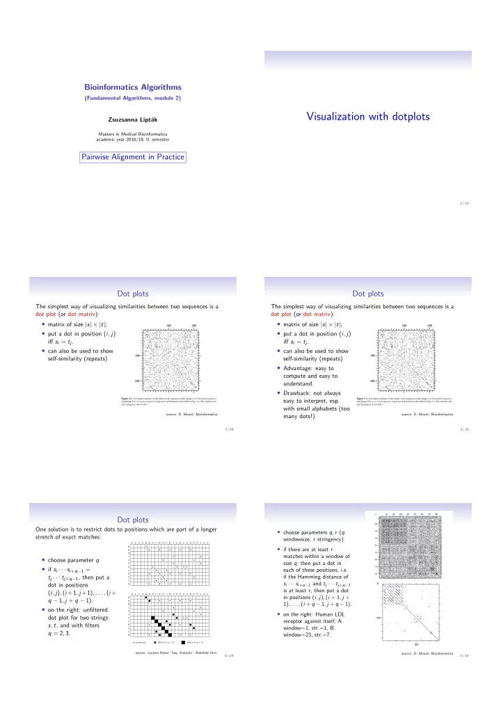
Dot plots

The simplest way of visualizing similarities between two sequences is a dot plot (or dot matrix):

• matrix of size |s| × |t|;
• put a dot in position (i, j)

iff si = tj.

• can also be used to show

self-similarity (repeats)

Figure 3.5. Dot matrix analysis of the amino acid sequences of the phage cI (horizontal sequence) and phage P22 c2 (vertical sequence) repressors performed as described in Fig. 3.4. The window size and stringency were both 1.

source: D. Mount: Bioinformatics 3 / 19

Dot plots

The simplest way of visualizing similarities between two sequences is a dot plot (or dot matrix):

• matrix of size |s| × |t|;
• put a dot in position (i, j)

iff si = tj.

• can also be used to show

self-similarity (repeats)

• Advantage: easy to

compute and easy to understand.

• Drawback: not always

easy to interpret, esp. with small alphabets (too many dots!)

Figure 3.5. Dot matrix analysis of the amino acid sequences of the phage cI (horizontal sequence) and phage P22 c2 (vertical sequence) repressors performed as described in Fig. 3.4. The window size and stringency were both 1.

source: D. Mount: Bioinformatics 3 / 19

Dot plots

One solution is to restrict dots to positions which are part of a longer stretch of exact matches:

• choose parameter q
• if si · · · si+q−1 =

tj · · · tj+q−1, then put a dot in positions (i, j), (i +1, j +1), . . . , (i + q − 1, j + q − 1).

• on the right: unfiltered

dot plot for two strings s, t, and with filters q = 2, 3.

F L U O R E S C E N C E I S E S S E N T I A L R E M I N I S C E N C E

• F L U O R E S C E N C E

I S E S S E N T I A L R E M I N I S C E N C E

• unfiltered

filtered (q = 2) filtered (q = 3)

source: Lecture Notes ”Seq. Analysis”, Bielefeld Univ. 4 / 19

• choose parameters q, r (q

windowsize, r stringency)

• if there are at least r

matches within a window of size q, then put a dot in each of these positions, i.e. if the Hamming distance of si · · · si+q−1 and tj · · · tj+q−1 is at least r, then put a dot in positions (i, j), (i + 1, j + 1), . . . , (i + q − 1, j + q − 1).

• on the right: Human LDL

receptor against itself; A. window=1, str.=1, B. window=23, str.=7.

source: D. Mount: Bioinformatics 5 / 19

Database search with BLAST

6 / 19

Database search

• Until now: compare two sequences
• how similar/different are they? (score/value)
• where are the similarities/differences? (alignment)
• Now: compare one sequence to a database (i.e. to many sequences)

7 / 19

Database search

Goal:

Identifying sequences in the DB which have high local similarity with the query.

• We know how to do this: Smith-Waterman DP-algorithm.
• But: too slow!

8 / 19

Say all sequences have length n (query t and all DB seq’s), and there are r sequences in the DB.

• time of exact solution (Smith-Waterman): O(r · n2)

9 / 19

Say all sequences have length n (query t and all DB seq’s), and there are r sequences in the DB.

• time of exact solution (Smith-Waterman): O(r · n2)

Example

• UniProt/SwissProt (protein database): 548 454 sequences,

195 409 447 aa’s (avg. length 350 aa’s)

version 29/04/15

• NCBI Genbank (nucleotide database): 182 188 746 sequences,

189 739 230 107 nucleotides (avg. length 1041 nucl.) April 2015, no WGS So we would get something like 350 · 350 · 548454 = 67 185 615 000 = about 67 billion (67 · 109) steps, which takes 18 hours on a computer that performs 1 million operations per second (for UniProt), and 197 434 482 454 026 (≈ 1.9 · 1012), about 6 years, for Genbank. And still about 1 hour on a computer performing 1 billion operations per second.

9 / 19

Say all sequences have length n (query t and all DB seq’s), and there are r sequences in the DB.

• time of exact solution (Smith-Waterman): O(r · n2)

Example

• UniProt/SwissProt (protein database): 548 454 sequences,

195 409 447 aa’s (avg. length 350 aa’s)

version 29/04/15

• NCBI Genbank (nucleotide database): 182 188 746 sequences,

189 739 230 107 nucleotides (avg. length 1041 nucl.) April 2015, no WGS So we would get something like 350 · 350 · 548454 = 67 185 615 000 = about 67 billion (67 · 109) steps, which takes 18 hours on a computer that performs 1 million operations per second (for UniProt), and 197 434 482 454 026 (≈ 1.9 · 1012), about 6 years, for Genbank. And still about 1 hour on a computer performing 1 billion operations per second. And this is for one query only!

9 / 19

BLAST: Basic Local Alignment Search Tool

• Altschul et al. 1990, 1997 (among the most highly cited papers in

bioinformatics)

• looks for sequences in a database with high local similarity to query
• heuristic algorithm
• solid mathematical foundations (Karlin-Altschul statistics)
• extremely successful, now the database search tool (“to blast a

sequence against a database”)

• NCBI1 Blast at:

http://blast.ncbi.nlm.nih.gov/Blast.cgi

1NCBI = National Center for Biotechnology Information 10 / 19

Basic idea

Basic idea

If there is a good local alignment between two sequences, then this local alignment is likely to contain a pair of short substrings with high score when aligned without gaps.

Basic steps of BLAST

• 1. create list of high-scoring words with query
• 2. scan DB for these words (called seeds)
• 3. extend seeds in both directions to form good gapless local alignment

(locally maximal segment pairs = HSPs)

11 / 19

Parameters

The original BLAST uses the following parameters:

• w: word size (length of high-scoring words)

default for DNA: w = 11, for protein: w = 3.

• T: threshold for high-scoring words
• d: absolute drop from highest scoring extension so far, or

α: relative drop from highest scoring extension so far

• S: threshold for retaining HSPs

Underlying theory of MSPs (maximal segment pairs) allows to estimate the highest MSP score S at which chance similarities are probable. HSPs are an approximation of MSPs; BLAST retains only those HSPs from the last step whose score is above this threshold S.

12 / 19

Step 1: create list of high-scoring words

Let t be the query sequence. A word v of length w is called high-scoring if there exists a substring u of t s.t. score(u, v) ≥ T, where score(u, v) = Pw

i=1 f (ui, vi), the score of a

gapless alignment of u with v. In other words, high-scoring words are the elements of the set H =

|t|−w+1

[

i=1

N(ti · · · ti+w−1), where N(u) = {v : score(u, v) ≥ T} is the T-neighborhood of the word u. Note that not every w-substring of t is necessarily element of H (its score with itself could be below T). Also, a word v could be high-scoring thanks to its closeness to two different w-substrings of t.

13 / 19

Example

• w = 3, T = 22, using the PAM250 scoring matrix.
• t = . . . FRNFKCVDNYAWC . . .
• Step 1:

Generate high-scoring words. For example, score(FKC,FKC) = 26, score(FKC,FRC) = 24, score(FKC,FNC) = 22, score(FKC,YKC) = 24, score(FKC,YRC) = 22. . . — these are all high-scoring w.r.t. the substring FKC of t. Others are high-scoring w.r.t. another substring of t, e.g. FWC is high-scoring because score(FWC,AWC) = 26 (but not w.r.t. FKC, since score(FWC,FKC) = 18 < 21).

• So for each high-scoring word v ∈ H, we need a list of positions i in t

s.t. score(v, ti · · · ti+w−1) ≥ T.

• Some high-scoring words are then: FKC,FRC,FNC,YKC,YRC, . . . (w.r.t.

FKC), AWC,FWC,DWC,LWC, . . . (wr.t. AWC), . . .

14 / 19

Step 2: Find occurrences of high-scoring words in DB sequences

Step 2. For each high-scoring word v, find all occurrences of v in the DB (i.e. in some sequence sk in the DB). These are called seeds.

Example (cont.)

Let v = FRC, which is high-scoring w.r.t. FKC (substring of t). Let the following be a sequence from the DB: s = . . . RNKDQKFRCAVDYAGM . . .

N.B.: This can be done efficiently using dedicated data structures for strings (e.g. generelized suffix array); this is beyond the scope of this course.

15 / 19

Step 3: Try to extend seeds

Step 3. For each of these seeds, try to extend to an HSP: Let sk have an

• ccurrence of a high-scoring word v (w.r.t. u = ti · · · ti+w−1) in position j,

then we already know that ✓ titi+1 . . . ti+w−1 sk

j sk j+1 . . . sk j+w−1

◆ is a gapless alignment with score ≥ T. We try to extend it in both directions to get a good HSP/MSP.

16 / 19

Example (cont.)

t = . . .FRNFKCVDNYAWC . . . s = . . . RNKDQKFRCAVDYAGM . . . We extend this alignment to both sides character by character, to get a good gapless local alignment. When do we stop? We could stop whenever we find a negative score (here at f (V, A) = −2); however, then we could miss a good longer local alignment. So one possibility is to set a maximum difference d to current best score: extend until score < X − d, where X = highest-score-seen-so-far. Another is to set a relative difference α: we extend until we drop below (1 − α)X. E.g. for α = 0.1 we get: ✓RNFKCVDNYA QKFRCAVDYA ◆ with score 38. This local alignment is now retained iff 38 > S.

17 / 19

BLAST2

Some of the main changes in BLAST2 (Altschul el al. 1997)

• start with two seeds instead of one, not too far apart
• gapped alignments
• extension of statistical theory to HSPs (high-scoring segment pairs)

Note: All versions of BLAST include many complex pre- and postprocessing steps, optimizations, . . . These are explained in the cited papers, and followup publications. Here we only looked at the basic ideas

• f the algorithm.

18 / 19

The NCBI BLAST website

• Different versions of BLAST, depending on the task (nucl-nucl:

blastn, megablast, . . . , prot-prot: blastp, psi-blast, nucl-prot: blastx, prot-nucl: tblastn, . . . )

• Different databases (nucl vs. prot, different organisms, different types
• f db, different levels of assembly, . . . )
• Very good explanations and help pages!

19 / 19