today dsp big picture
play

Today DSP Big Picture Digital filters and signal processing Filter - PDF document

Today DSP Big Picture Digital filters and signal processing Filter examples and properties FIR filters Filter design Implementation issues DACs PWM
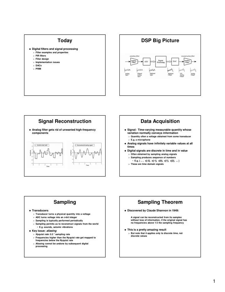
 Signal Reconstruction Data Acquisition Analog filter gets rid of


  1. Today DSP Big Picture � Digital filters and signal processing � Filter examples and properties � FIR filters � Filter design � Implementation issues � DACs � PWM Signal Reconstruction Data Acquisition � Analog filter gets rid of unwanted high-frequency � Signal: Time-varying measurable quantity whose components variation normally conveys information � Quantity often a voltage obtained from some transducer � E.g. a microphone � Analog signals have infinitely variable values at all times � Digital signals are discrete in time and in value � Often obtained by sampling analog signals � Sampling produces sequence of numbers • E.g. { ... , x[-2], x[-1], x[0], x[1], x[2], ... } � These are time domain signals Sampling Sampling Theorem � Transducers � Discovered by Claude Shannon in 1949: � Transducer turns a physical quantity into a voltage � ADC turns voltage into an n -bit integer A signal can be reconstructed from its samples without loss of information, if the original signal has � Sampling is typically performed periodically no frequencies above 1/2 the sampling frequency � Sampling permits us to reconstruct signals from the world • E.g. sounds, seismic vibrations � This is a pretty amazing result � Key issue: aliasing � But note that it applies only to discrete time, not � Nyquist rate : 0.5 * sampling rate discrete values � Frequencies higher than the Nyquist rate get mapped to frequencies below the Nyquist rate � Aliasing cannot be undone by subsequent digital processing 1

  2. Aliasing Details No Aliasing � Let N be the sampling rate and F be a frequency found in the signal � Frequencies between 0 and 0.5*N are sampled properly � Frequencies >0.5*N are aliased • Frequencies between 0.5*N and N are mapped to (0.5*N)- F and have phase shifted 180 � • Frequencies between N and 1.5*N are mapped to f-N with no phase shift • Pattern repeats indefinitely � Aliasing may or may not occur when N == F*2*X where X is a positive integer 1 kHz Signal, No Aliasing Aliasing More Aliasing N == 2*F Example 2

  3. Avoiding Aliasing Signal Processing Pragmatics Increase sampling rate 1. Not a general-purpose solution � • White noise is not band-limited • Faster sampling requires: – Faster ADC – Faster CPU – More power More RAM for buffering – Filter out undesirable frequencies before sampling 2. using analog filter(s) � This is what is done in practice � Analog filters are imperfect and require tradeoffs Aliasing in Space Point vs. Supersampling � Spatial sampling incurs aliasing problems also � Example: CCD in digital camera samples an image in a grid pattern � Real world is not band-limited � Can mitigate aliasing by increasing sampling rate Point sampling 4x4 Supersampling Samples Pixel Digital Signal Processing Assumptions � Basic idea Signal sampled at fixed and known rate f s 1. � Digital signals can be manipulated losslessly � I.e., ADC driven by timer interrupts � SW control gives great flexibility � DSP examples Aliasing has not occurred 2. � Amplification or attenuation � I.e., signal has no significant frequency components greater than 0.5*f s � Filtering – leaving out some unwanted part of the signal These have to be removed before ADC using an analog � � Rectification – making waveform purely positive filter � Modulation – multiplying signal by another signal � Non-significant signals have amplitude smaller than the • E.g. a high-frequency sine wave ADC resolution 3

  4. Filter Terms for CS People Simple Digital Filters � Low pass – lets low frequency signals through, � y(n) = 0.5 * (x(n) + x(n-1)) suppresses high frequency � Why not use x(n+1)? � High pass – lets high frequency signals through, � y(n) = (1.0/6) * (x(n) + x(n-1) + x(n-2) + … + y(n-5) ) suppresses low frequency � y(n) = 0.5 * (x(n) + x(n-3)) � Passband – range of frequencies passed by a filter � y(n) = 0.5 * (y(n-1) + x(n)) � Stopband – range of frequencies blocked � What makes this one different? � Transition band – in between these � y(n) = median [ x(n) + x(n-1) + x(n-2) ] Gain vs. Frequency Useful Signals 1.5 y(n) =(y(n-1)+x(n))/2 � Step: Step 1 y(n) =(x(n)+x(n-1))/2 � …, 0, 0, 0, 1, 1, 1, … s(n) y(n) =(x(n)+x(n-1)+x(n-2)+ 1.0 x(n-3)+x(n-4)+x(n-5))/6 Gain y(n) =(x(n)+x(n-3))/2 -3 -2 -1 0 1 2 3 0.5 � Impulse: Impulse 1 i(n) � …, 0, 0, 0, 1, 0, 0, … 0.0 0.0 0.1 0.2 0.3 0.4 0.5 frequency f/fs -3 -2 -1 0 1 2 3 Step Response Impulse Response 1 1 0.8 0.8 step input impulse input Response Response 0.6 FIR 0.6 FIR 0.4 IIR 0.4 IIR median median 0.2 0.2 0 0 0 1 2 3 4 5 0 1 2 3 4 5 sample number, n sample number, n 4

  5. FIR Filters Moving Average Example � Finite impulse response � Filter “remembers” the arrival of an impulse for a finite time � Designing the coefficients can be hard � Moving average filter is a simple example of FIR FIR in C Implementation Issues SAMPLE fir_basic (SAMPLE input, int ntaps, � Usually done with fixed-point const SAMPLE coeff[], � How to deal with overflow? SAMPLE z[]) � A few optimizations { � Put coefficients in registers z[0] = input; � Put sample buffer in registers SAMPLE accum = 0; � Block filter for (int ii = 0; ii < ntaps; ii++) { • Put both samples and coefficients in registers accum += coeff[ii] * z[ii]; • Unroll loops } � Hardware-supported circular buffers for (ii = ntaps - 2; ii >= 0; ii--) { z[ii + 1] = z[ii]; � Creating very fast FIR implementations is important } return accum; } Filter Design Filter Design in Matlab � Where do coefficients come from for the moving � Matlab has excellent filter design support average filter? � C = firpm (N, F, A) � In general: � N = length of filter - 1 Design filter by hand � F = vector of frequency bands normalized to Nyquist 1. Use a filter design tool � A = vector of desired amplitudes 2. � firpm uses minimax – it minimizes the maximum � Few filters designed by hand in practice deviation from the desired amplitude � Filters design requires tradeoffs between Filter order 1. Transition width 2. Peak ripple amplitude 3. � Tradeoffs are inherent 5

  6. Filter Design Examples Example Filter Response f = [ 0.0 0.3 0.4 0.6 0.7 1.0]; a = [ 0 0 1 1 0 0]; fil1 = firpm( 10, f, a); fil2 = firpm( 17, f, a); fil3 = firpm( 30, f, a); fil4 = firpm(100, f, a); fil2 = Columns 1 through 8 -0.0278 -0.0395 -0.0019 -0.0595 0.0928 0.1250 -0.1667 -0.1985 Columns 9 through 16 0.2154 0.2154 -0.1985 -0.1667 0.1250 0.0928 -0.0595 -0.001 Columns 17 through 18 -0.0395 -0.0278 Testing an FIR Filter � Impulse test � Feed the filter an impulse � Output should be the coefficients � Step test � Feed the filter a test � Output should stabilize to the sum of the coefficients � Sine test � Feed the filter a sine wave � Output should have the expected amplitude 6

  7. Digital to Analog Converters Pulse Width Modulation � Opposite of an ADC � PWM answers the question: How can we generate � Available on-chip and as separate modules analog waveforms using a single-bit output? � Also not too hard to build one yourself � Can be more efficient than DAC � DAC properties: � Precision: Number of distinguishable alternatives • E.g. 4092 for a 12-bit DAC � Range: Difference between minimum and maximum output (voltage or current) � Speed: Settling time, maximum output rate � LPC2129 has no built-in DACs Summary PWM � Filters and other DSP account for a sizable percentage of embedded system activity � Approximating a DAC: � Filters involve unavoidable tradeoffs between � Set PWM period to be much lower than DAC period � Adjust duty cycle every DAC period � Filter order � Transition width � PWM is starting to be used in audio equipment � Peak ripple amplitude � Important application of PWM is in motor control � In practice filter design tools are used � No explicit filter necessary – inertia makes the motor its own low-pass filter � We skipped all the theory! � Lots of ECE classes on this 7

Download Presentation
Download Policy: The content available on the website is offered to you 'AS IS' for your personal information and use only. It cannot be commercialized, licensed, or distributed on other websites without prior consent from the author. To download a presentation, simply click this link. If you encounter any difficulties during the download process, it's possible that the publisher has removed the file from their server.

Recommend


More recommend