To Do To Do Computer Graphics (Spring 2008) Computer Graphics - PDF document

To Do To Do Computer Graphics (Spring 2008) Computer Graphics (Spring 2008) � Work on HW 3, do well � Start early on HW 4 COMS 4160, Lecture 15: Illumination and Shading http://www.cs.columbia.edu/~cs4160 Course Outline Course Outline Course Outline Course Outline � 3D Graphics Pipeline � 3D Graphics Pipeline Rendering Rendering Modeling Modeling (Creating, shading images from (Creating, shading images from (Creating 3D Geometry) (Creating 3D Geometry) geometry, lighting, materials) geometry, lighting, materials) Unit 1: Transformations Unit 4: Shading, Ray Trace Weeks 1,2. Ass 1 due Feb 14 Weeks 8,9. Unit 3: OpenGL Ass 4 due May 4 Weeks 5-7. Unit 2: Spline Curves Ass 3 due Apr 1 Weeks 3,4. 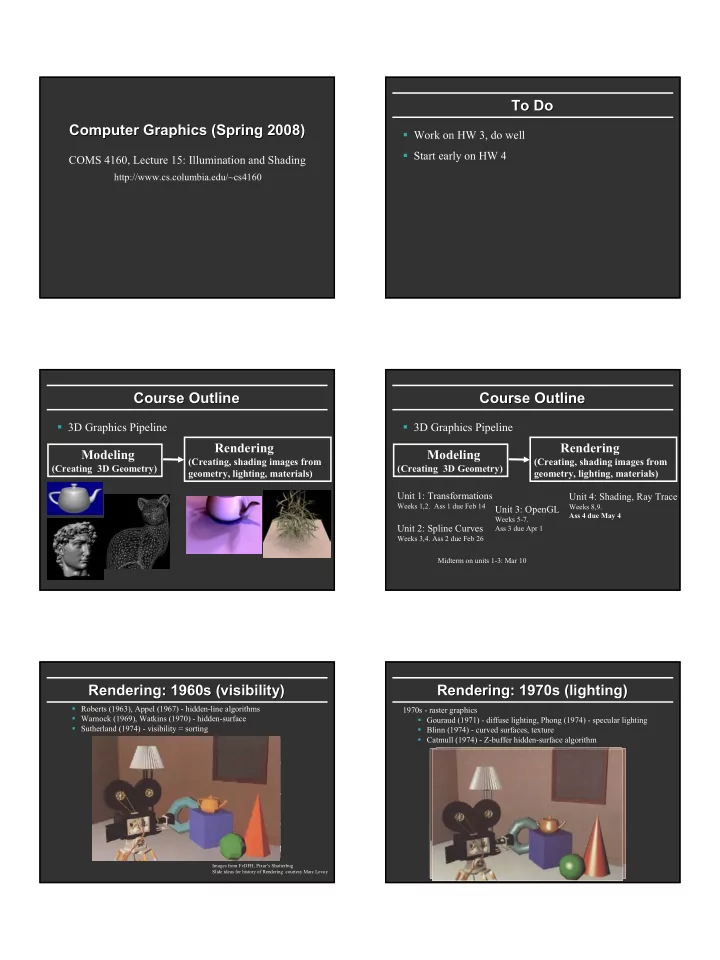Ass 2 due Feb 26 Midterm on units 1-3: Mar 10 Rendering: 1960s (visibility) Rendering: 1960s (visibility) Rendering: 1970s (lighting) Rendering: 1970s (lighting) � Roberts (1963), Appel (1967) - hidden-line algorithms 1970s - raster graphics � Warnock (1969), Watkins (1970) - hidden-surface � Gouraud (1971) - diffuse lighting, Phong (1974) - specular lighting � Sutherland (1974) - visibility = sorting � Blinn (1974) - curved surfaces, texture � Catmull (1974) - Z-buffer hidden-surface algorithm Images from FvDFH, Pixar’s Shutterbug Slide ideas for history of Rendering courtesy Marc Levoy

Outline Outline Rendering (1980s, 90s: Global Illumination) Rendering (1980s, 90s: Global Illumination) early 1980s - global illumination � Preliminaries � Whitted (1980) - ray tracing � Basic diffuse and Phong shading � Goral, Torrance et al. (1984) radiosity � Kajiya (1986) - the rendering equation � Gouraud, Phong interpolation, smooth shading � Formal reflection equation For today’s lecture, slides and chapter 9 in textbook Motivation Motivation Linear Relationship of Light Linear Relationship of Light � Objects not flat color, perceive shape with appearance � Light energy is simply sum of all contributions ∑ = I I � Materials interact with lighting k k � Compute correct shading pattern based on lighting � Terms can be calculated separately and later added � This is not the same as shadows (separate topic) together: � multiple light sources � Some of today’s lecture review of last OpenGL lec. � multiple interactions (diffuse, specular, more later) � Idea is to discuss illumination, shading independ. OpenGL � multiple colors (R-G-B, or per wavelength) � Today, initial hacks (1970-1980) � Next lecture: formal notation and physics General Considerations General Considerations Diffuse Lambertian Diffuse Lambertian Term Term Surfaces are described as having a position, and a normal at � Rough matte (technically Lambertian) surfaces every point. � Not shiny: matte paint, unfinished wood, paper, … N 1 � Light reflects equally in all directions (x 1 ,y 1 ,z 1 ) N 2 � Obey Lambert’s cosine law (x 2 ,y 2 ,z 2 ) � Not exactly obeyed by real materials N • I ∼ N L Other vectors used -L � L = vector to the light source light position minus surface point position � E = vector to the viewer (eye) viewer position minus surface point position

Meaning of negative dot products Phong Illumination Model Illumination Model Meaning of negative dot products Phong � If (N dot L) is negative, then the light is behind the surface, � Specular or glossy materials: highlights and cannot illuminate it. � Polished floors, glossy paint, whiteboards � For plastics highlight is color of light source (not object) � For metals, highlight depends on surface color � Really, (blurred) reflections of light source � If (N dot E) is negative, then the viewer is looking at the underside of the surface and cannot see it’s front-face. � In both cases, I is clamped to Zero. Roughness Idea of Idea of Phong Phong Illumination Illumination Phong Phong Formula Formula � Find a simple way to create highlights that are view- I ∼ ( R E i ) p dependent and happen at about the right place R � Not physically based -L E � Use dot product (cosine) of eye and reflection of light direction about surface normal � Alternatively, dot product of half angle and normal � Raise cosine lobe to some power to control sharpness R = = − + ? R L 2( L N N i ) or roughness Outline Outline Alternative: Half- Alternative: Half -Angle ( Angle (Blinn Blinn- -Phong Phong) ) ) p � Preliminaries I ∼ ( N H i � Basic diffuse and Phong shading H N � Gouraud, Phong interpolation, smooth shading � Formal reflection equation Not in text. If interested, look at FvDFH pp 736-738 � In practice, both diffuse and specular components for most materials

Vertex Shading Triangle Meshes as Approximations Triangle Meshes as Approximations Vertex Shading � Most geometric models are large collections of � We know how to calculate the light intensity given: triangles. � surface position � normal � Triangles have 3 vertices, each with a position, color, � viewer position normal, and other parameters (such as n for Phong � light source position (or direction) reflection). � The triangles are an approximation to the actual � 2 ways for a vertex to get its normal: surface of the object. � given when the vertex is defined. � take all the normals from faces that share the vertex, and average them. Coloring Inside the Polygon Coloring Inside the Polygon Flat vs. Gouraud Flat vs. Gouraud Shading Shading � How do we shade a triangle between it’s vertices, where we aren’t given the normal? � Inter-vertex interpolation can be done in object space (along the face), but it is simpler to do it in image glShadeModel(GL_FLAT) glShadeModel(GL_SMOOTH) space (along the screen). Flat - Determine that each face has a single normal, and color the entire face a single value, based on that normal. Gouraud – Determine the color at each vertex, using the normal at that vertex, and interpolate linearly for the pixels between the vertex locations. Gouraud Gouraud Shading Shading – – Details Details Gouraud Gouraud and Errors and Errors − + − I y ( y ) I ( y y ) = I 1 s 2 2 1 s � I 1 = 0 because (N dot E) is negative. a − y y 1 2 − + − I y ( y ) I ( y y ) � I 2 = 0 because (N dot L) is negative. = I 1 s 3 3 1 s I b − y y 1 1 3 y � Any interpolation of I 1 and I 2 will be 0. 1 I ( x − x ) + I ( x − x ) = a b p b p a I p − x x b a I I I Scan line a p b y s y I 2 2 y I 3 I 1 = 0 I 2 = 0 3 area of desired Actual implementation efficient: difference highlight equations while scan converting

2 Phongs Phongs make a Highlight make a Highlight 2 Problems with Interpolated Shading Problems with Interpolated Shading � Besides the Phong Reflectance model (cos n ), there is a Phong � Silhouettes are still polygonal Shading model. � Interpolation in screen, not object space: perspective distortion � Phong Shading: Instead of interpolating the intensities between � Not rotation or orientation-independent vertices, interpolate the normals . � How to compute vertex normals for sharply curving surfaces? � The entire lighting calculation is performed for each pixel, based on the interpolated normal. (OpenGL doesn’t do this, but you can with current programmable shaders) � But at end of day, polygons is mostly preferred to explicitly representing curved objects like spline patches for rendering I 1 = 0 I 2 = 0 Motivation Outline Outline � Preliminaries • Lots of ad-hoc tricks for shading � Basic diffuse and Phong shading – Kind of looks right, but? • Physics of light transport � Gouraud, Phong interpolation, smooth shading – Will lead to formal reflection equation � Formal reflection equation • One of the more formal lectures – But important to solidify theoretical framework

Radiance • Power per unit projected area perpendicular to the ray per unit solid angle in the direction of the ray • Symbol: L(x, ω ) (W/m 2 sr) • Flux given by d Φ = L(x, ω ) cos θ d ω dA Radiance properties • Radiance is constant as it propagates along ray – Derived from conservation of flux – Fundamental in Light Transport. Φ = ω = ω = Φ d L d dA L d dA d 1 1 1 2 2 2 1 2 ω = 2 ω = 2 d dA r d dA r 1 2 2 1 dA dA ω = = ω d dA 1 2 d dA 1 1 2 2 r 2 ∴ = L L 1 2 Radiance properties • Sensor response proportional to radiance (constant of proportionality is throughput) – Far away surface: See more, but subtends smaller angle – Wall equally bright across viewing distances Consequences – Radiance associated with rays in a ray tracer – Other radiometric quants derived from radiance