logistics
play

Logistics Checkpoint 1 all graded Material Properties Grades / - PDF document

Logistics Checkpoint 1 all graded Material Properties Grades / comments on mycourses Project Proposals all graded Comments in mycourses List of projects on course Web site Reminder Illumination Models / BRDFs Readings:


  1. Logistics  Checkpoint 1 all graded Material Properties  Grades / comments on mycourses  Project Proposals all graded  Comments in mycourses  List of projects on course Web site  Reminder Illumination Models / BRDFs  Readings: undergrad - 1 / week  Grads: - 1/ class  Checkpoint 2  Due Monday  Questions? Plan for today 
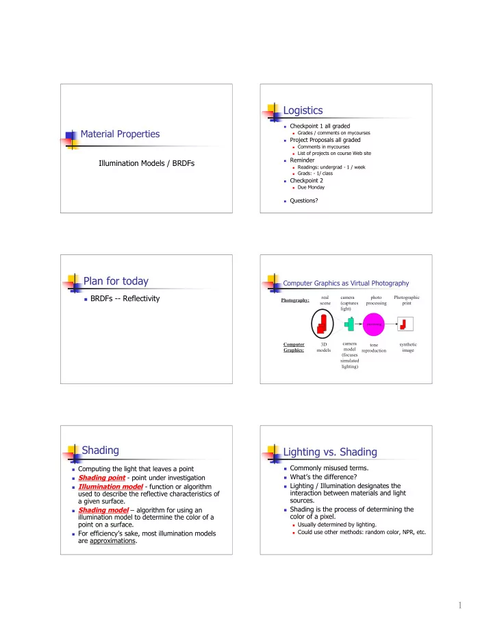
Computer Graphics as Virtual Photography  BRDFs -- Reflectivity real camera photo Photographic Photography: scene (captures processing print light) processing camera Computer 3D synthetic tone model Graphics: models image reproduction (focuses simulated lighting) Shading Lighting vs. Shading  Commonly misused terms.  Computing the light that leaves a point  What’s the difference?  Shading point - point under investigation  Lighting / Illumination designates the  Illumination model - function or algorithm interaction between materials and light used to describe the reflective characteristics of sources. a given surface.  Shading is the process of determining the  Shading model – algorithm for using an color of a pixel. illumination model to determine the color of a point on a surface.  Usually determined by lighting.  Could use other methods: random color, NPR, etc.  For efficiency’s sake, most illumination models are approximations. 1

  2. Bi-directional Reflectance Functions (BRDF) Reflections  Ambient – light uniformly incident from the environment  Diffuse – light scattered equally in all directions  Ambient and Diffuse – color of material plays a part  Specular – highlights connected with mirrorness  Specular – mostly color of light BRDF BRDF Geometry  Bi-directional Reflectance Function BRDF f ( , , , ) = � � � � r i i r r At a given point, gives relative reflected illumination in any direction with respect to incoming illumination coming from any direction; Note: The θ ’s are elevation, ϕ ’s are measured about the surface normal. The i ’s refer to the incident ray; the r ’s to the reflected ray. BRDF BRDF  Can return any positive value.  Simplifying Assumptions wrt the BRDF  Generally wavelength specific.  Light enters and leaves from the same point.  Not necessarily true  Subsurface scattering BRDF = f ( , , , , ) � � � � �  Skin, marble r i i r r  Light of a given wavelength will only reflect back light of that same wavelength  Not necessarily true  Light Interference  Oily patches, peacock feathers 2

  3. Illumination Models Illumination Modeling  Four approaches  Illumination model - function or  Simplistic algorithm used to describe the reflective  Based on physics, abiet with many assumptions characteristics of a given surface.  Heuristic  Revise to…  The kludge!  Usually simple, yet not physically based  function or algorithm used in  Simulation approximating the BRDF.  Employ physical model  More complex than heuristic, but more accurate  Empirical  Use measured samples Illumination Models Reflection and color  Illumination Models and Viewing  Color “response” is based on color that reaches the eye or sensor Direction  Generally, BRDFs are independent of  http://www.cs.brown.edu/exploratories/freeS viewing direction oftware/repository/edu/brown/cs/exploratorie  Most Illumination models take viewing s/applets/spectrum/reflection_guide.html direction into consideration  http://www.cs.brown.edu/exploratories/freeS oftware/repository/edu/brown/cs/exploratorie s/applets/spectrum/two_materials_java_brow ser.html Reflections Illumination Models  Ambient – light uniformly incident from the  Geometry environment N  Diffuse – light scattered equally in all directions V H  Ambient and Diffuse – color of material plays a part viewer normal Half-way  Specular – highlights connected with mirrorness R  Specular – mostly color of light S reflection source 3

  4. Illumination Models Illumination Models  Recall from Linear Algebra  Geometry  N - normal vector u  S - direction of incoming light θ  R - direction of perfect mirror reflection v  H - halfway between light direction and viewing direction. u v u v cos • = �  V - viewing direction. Just one reason to normalize! Illumination Modeling Illumination Models  Four approaches  BRDF Viewer  Simplistic  bv by Szymon Rusinkiewicz (Princeton)  Lamertian  http://graphics.stanford.edu/~smr/brdf/bv  Heuristic  SGI, Linux, and Java versions although not  Phong readily available for Java. I have it, if you  Simulation want it, and you’ll need to load Java3D as  Cook-Torrance well!  Empirical  Use measured samples Simplistic Lambert’s Cosine Law  Lambertian Model  The reflected luminous intensity in any direction from a perfectly  Perfectly diffuse surface diffusing surface varies as the  reflection is constant in all directions (k d ) cosine of the angle between the  Independent of viewer direction direction of incident light and the  Based on Lambert’s cos law. normal vector of the surface.  Sometimes mistakenly attributed to Gouraud.  Intuitively  Gouraud didn’t introduce a new lighting model, just a  cross-sectional area of shading method. the “beam” intersecting an element of surface area is smaller for greater angles with the normal. 4

  5. Lambertian Model Lambertian Model  Lambert Model  BRDF Viewer http://graphics.stanford.edu/~smr/brdf/ bv L ( V ) L S k cos = � L ( V ) L k ( N S ) = • d S d Those Were the Days Phong Model  (Or: how not to motivate a 21 st century  Phong Model computer graphics paper.)  introduces specular (mirror-like) reflections  “In trying to improve the quality of the  Viewer direction becomes more important synthetic images, we do not expect to be able  three components to display the object exactly as it would appear  ambient - background light (k a ) in reality, with texture, overcast shadows, etc. We hope only to display an image that  diffuse - Lambertian reflection (k d ) approximates the real object closely enough to  specular – mirror-like reflection(k s ) provide a certain degree of realism.” – Bui Tuong Phong, 1975 Phong Model Phong-Blinn Model  Uses halfway angle rather than reflected ∑ ∑ k L ( V ) = k L + k L ( S • N) + k L ( R • V) e a a d i i s i i i i ∑ ambient ∑ = + • + • k diffuse specular L ( V ) k L k L ( S N) k L ( H N) e a a d i i s i i i i ambient Note: L n are radiance terms, include both light and material info diffuse specular 5

  6. Phong-Blinn Model Physically based  BRDF Viewer  based on physics of a surface  Actually developed by Torrance & Sparrow, physicists.  Jim Blinn was the first to apply to CG http://graphics.stanford.edu/~smr/brdf/  Cook & Torrance’s was the first complete implementation bv  components  microfacet model - describes geometry of surface  And how much the microfacets shadow each other.  Fresnel term - describes reflectance  Roughness - describes microfacet distribution. Break? Cook-Torrance Model Cook-Torrance Model  Microfacets  Microfacets  surface is composed of V shaped grooves (microfacets)  Light interactions with microfacets  Reflect - causes specular reflections  Scatter - causes diffuse reflections Cook-Torrance Model Cook-Torrance Model  Microfacets – GeometryTerm  Fresnel Equation for polarized light  Some microfacets may shadow others  Describes reflectance as a function of:  Wavelength of incident light ( λ )  Index of refraction ( η ( λ ))  Extinction coefficient (ease at which wave can penetrate a surface) ( κ ( λ ))  Angle of incidence ( θ )  2 ( N • H)(N • V) 2 ( N • H)(N • S)  G = min 1 , ,   (V • H) (V • H)   Note: S from before is the L in these diagrams 6

  7. Cook-Torrance Model Cook-Torrance Model  Fresnel equations for polarized light  Fresnel 2 2 2 a + b − 2 a cos θ + cos θ Perpendicular component  If all quantities known, use Fresnel = Fs 2 + 2 + θ + 2 θ equations a b 2 a cos cos  If not, approximate using reflectance off 2 2 2 2 a b 2 a sin tan sin tan Parallel component + � � � + � � F F normal = p s 2 2 2 2 a b 2 a sin tan sin tan + + � � + � �  See [Glassner] or [Cook/Torrance81] for details a, b are functions 1 1 F F F of η , κ , and θ = + s p 2 2 η , κ are functions F is total reflectance of λ Cook-Torrance Model Cook-Torrance Model  Roughness  Roughness  Characterizes the distribution of the slopes of the microfacets  Roughness parameter, m  m between 0 -1  small m - smooth surface, specular reflectance 2 2 − ((tan α ) / m ) − ( α / m ) e D = ce  large m - rough surface, diffuse reflectance D = 2 4 m cos α  Statistical models Gaussian Model Beekman Model c is arbitrary constant Cook-Torrance Model Cook-Torrance Model  Roughness  Putting it all together f = sf + df r s d specular diffuse total reflectance 1 × × 1 F D G f = f s = d � π ( N • S)(N • V) Where D is the roughness function, F is the Fresnel function, and G is the geometrical attenuation factor from previous pages 7

Download Presentation
Download Policy: The content available on the website is offered to you 'AS IS' for your personal information and use only. It cannot be commercialized, licensed, or distributed on other websites without prior consent from the author. To download a presentation, simply click this link. If you encounter any difficulties during the download process, it's possible that the publisher has removed the file from their server.

Recommend


More recommend