The Road Ahead 1. Physical layer 2. Datalink layer Application - - PDF document

Page 1

CS 640: Introduction to Computer Networks

Aditya Akella Lecture 4 - Physical Layer Transmission and Link Layer Basics

The Road Ahead…

• 1. Physical layer
• 2. Datalink layer

introduction, framing, error coding, switched networks

• 3. Broadcast-networks,

home networking

Application Transport Network Datalink Physical

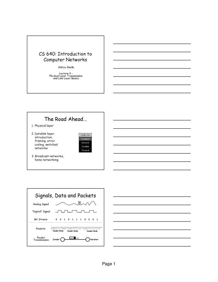
Signals, Data and Packets

Analog Signal “Digital” Signal Bit Stream

0 0 1 0 1 1 1 0 0 0 1

Packets

0100010101011100101010101011101110000001111010101110101010101101011010111001

Header/Body Header/Body Header/Body

Receiver Sender

Packet Transmission

Page 2

Binary data to Signals

• Encoding

– How to convert bits to “digital” signals – Very complex, actually – Error recovery, clock recovery,…

• Modulation: changing attributes of

signal to effect information transmissions

Modulation Schemes

Data Amplitude Modulation Frequency Modulation Phase Modulation

The Frequency Domain

• A signal can be viewed as a sum of sine waves of different

strengths.

• Every signal has an equivalent representation in the frequency

domain.

– What frequencies are present and their relative strength =

+ 1.3 X + 0.56 X + 1.15 X

Page 3

Why Do We Care?

• What limits the physical size of the network?
• How can multiple hosts communicate over the

same wire at the same time?

• How can I manage bandwidth on a

transmission medium?

• How do the properties of copper, fiber, and

wireless compare?

• How much bandwidth can I get out of a

specific wire (transmission medium)?

Transmission Channel Considerations

• Every medium supports

transmission in a certain frequency range.

– Outside this range, effects such as attenuation degrade the signal too much

• Transmission and reception

hardware will try to maximize the useful capacity in this frequency band.

– Tradeoffs between cost, distance, bit rate

• As technology improves,

these parameters change, even for the same wire.

– Thanks to our EE friends

Frequency

Good Bad

Loss/m

The Nyquist Limit

• A noiseless channel of width H can at most

transmit a binary signal at a rate 2 x H.

– E.g. a 3000 Hz channel can transmit data at a rate

• f at most 6000 bits/second

– Assumes constant frequency – Assumes AM – Assumes binary information transfer – Assumes no noise

Page 4

Past the Nyquist Limit

• More aggressive encoding can increase the

channel bandwidth

– Example: modems

• Same frequency - number of symbols per second
• Symbols have more possible values
• Use multiple modulation schemes together
• The channel bandwidth is determined by the

transmission medium and the quality of the transmitter and receivers

– Channel capacity increases over time

Capacity of a Noisy Channel

• Can’t add infinite symbols - you have to be able to tell

them apart. This is where noise comes in.

• Shannon’s theorem:

– C = B x log(1 + S/N) – C: maximum capacity (bps) – B: channel frequency range or bandwidth (Hz) – S/N: signal to noise ratio of the channel

• Often expressed in decibels (db). 10 log(S/N).
• Example:

– Local loop bandwidth: 3200 Hz – Typical S/N: 1000 (30db) – What is the upper limit on capacity?

Limits to Capacity

• Noise: “random” energy is

added to the signal.

• Attenuation: some of the

energy in the signal leaks away.

• Dispersion: attenuation and

propagation speed are frequency dependent.

– Changes the shape of the signal

• Effects limit the data rate that a channel can sustain.
• But affects different technologies in different ways
• Effects become worse with distance.
• Tradeoff between data rate and distance

Page 5 Supporting Multiple Channels

• Can multiple transmission channels coexist?

– Yes, if they transmit at a different frequency, or at a different time, or in a different part of the space.

• Space can limit use of wires or of transmit power of

wireless transmitters.

• Multiplexing

– Frequency multiplexing means that different users use a different part of the spectrum.

• Again, similar to radio: 95.5 versus 102.5 station

– Controlling time Time-division multiplexing: divide time into quanta

Frequency versus Time-division Multiplexing

• With frequency-division

multiplexing different users use different parts of the frequency spectrum.

– I.e. each user can send all the time at reduced rate – Example: roommates

• With time-division

multiplexing different users send at different times.

– I.e. each user can sent at full speed some of the time – Example: a time-share condo

• The two solutions can be

combined.

• Next.. A word about media

F r e q u e n c y Time

Frequency Bands Slot Frame

Copper Wire

• Unshielded twisted pair

– Two copper wires twisted - avoid antenna effect; differential – Grouped into cables: multiple pairs with common sheath – Category 3 (voice grade) versus Category 5 (Ethernet) – 100 Mbit/s up to 100 m, 1 Mbit/s up to a few km – Cost: ~ 10cents/foot; cheap

• Coax cables.

– One connector is placed inside the other connector – Holds the signal in place and keeps out noise – Gigabit up to a km

Page 6

Optical Fiber: Ray Propagation

lower index

• f refraction

core cladding (note: minimum bend radius of a few cm)

Optical Fiber Physical Constraints

1000

wavelength (nm) loss (dB/km)

1500 nm (~200 Thz) 0.0 0.5 1.0

tens of THz 1.3µ 1.55µ

LEDs Lasers

Fiber Types

• Multimode fiber

– Designed to carry multiple modes/rays each at slightly different angle – 62.5 or 50 micron core carries the multiple – used at 1.3 micron wavelength, usually LED source – subject to mode dispersion: different propagation modes travel at different speeds – typical limit: 1 Gbps at 100m

• Single mode

– 8 micron core carries a single mode – used at 1.3 or 1.55 microns, usually laser diode source – typical limit: 1 Gbps at 10 km or more – still subject to chromatic dispersion

Page 7 Regeneration and Amplification

• At end of span, either regenerate

electronically or amplify.

• Electronic repeaters are potentially slow, but

can eliminate noise.

• Amplification over long distances made

practical by erbium doped fiber amplifiers

• ffering up to 40 dB gain.
• Ex: 10 Gbps at 500 km.

source pump laser

Wavelength Division Multiplexing

• Send multiple wavelengths through the same fiber.

– Multiplex and demultiplex the optical signal on the fiber

• Each wavelength represents an optical carrier that

can carry a separate signal.

– E.g., 16 colors of 2.4 Gbit/second

• Like radio, but optical and much faster

Optical Splitter Frequency

Gigabit Ethernet: Physical Layer Comparison

Medium Transmit/receive Distance Copper 1000BASE-CX 25 m Twisted pair 1000BASE-T 100 m MM fiber 62 mm 1000BASE-SX 260 m 1000BASE-LX 500 m MM fiber 50 mm 1000BASE-SX 525 m 1000BASE-LX 550 m SM fiber 1000BASE-LX 5000 m

Page 8

Wireless Technologies

• Great technology: easy to use, no wires to install, convenient

mobility, ..

• High attenuation limits distances.

– Wave propagates out as a sphere (approximately) – Signal strength reduces quickly (1/distance)3

• High noise due to interference from other transmitters.

– Use MAC and other rules to limit interference

• E.g transmit power control

– Aggressive encoding techniques to make signal less sensitive to noise

• Don’t always work
• Other effects: multipath fading, security, ..
• Government tightly regulates spectrum usage

Summary So Far

• Bandwidth and distance of networks is limited by

physical properties of media.

– Attenuation, noise, …

• Network properties are determined by transmission

medium and transmit/receive hardware.

– Nyquist gives a rough idea of idealized throughput

• Multiple users can be supported using space, time, or

frequency division multiplexing.

• Properties of different transmission media.

Analog versus Digital

• Digital transmissions.

– Interpret the signal as a series of 1’s and 0’s – Hand over interpreted information to higher layers – E.g. data transmission over the Internet

• Analog transmission

– Do not interpret the contents – Just play out the signal – E.g broadcast radio

• Why digital transmission?

Page 9

Why Do We Need Encoding?

• Meet certain electrical constraints.

– Receiver needs enough “transitions” to keep track of the transmit clock – Avoid receiver saturation

• Create control symbols, besides regular data symbols.

– E.g. start or end of frame, escape, ... – Important in packet switching

• Error detection or error corrections.

– Some codes are illegal so receiver can detect certain classes of errors – Minor errors can be corrected by having multiple adjacent signals mapped to the same data symbol

• Encoding can be very complex, e.g. wireless.

Encoding

• Use two signals, high and low, to encode 0 and 1.
• Transmission is synchronous, i.e., a clock is used to

sample the signal.

– In general, the duration of one bit is equal to one or two clock ticks – Receiver’s clock must be synchronized with the sender’s clock

• Encoding can be done one bit at a time or in blocks of,

e.g., 4 or 8 bits.

Non-Return to Zero (NRZ)

• 1 -> high signal; 0 -> low signal
• Long sequences of 1’s or 0’s can cause problems:

– Hard to recover clock – Difficult to interpret 0’s and 1’s

V .85

• .85

1 1 1 1

Page 10

Non-Return to Zero Inverted (NRZI)

• 1 -> make transition; 0 -> signal stays the same
• Solves the problem for long sequences of 1’s, but

not for 0’s.

V .85

• .85

1 1 1 1

Ethernet Manchester Encoding

• Positive transition for 0, negative for 1
• XOR of NRZ with clock
• Transition every cycle communicates clock (but need 2 transition times

per bit)

• Problem: doubles the rate at which signal transitions are made

– Less efficient – Receiver has half the time to detect the pulse

V .85

• .85

1 1 .1µs

4B/5B Encoding

• Data coded as symbols of 5 line bits => 4 data

bits, so 100 Mbps uses 125 MHz.

– Uses less frequency space than Manchester encoding

• Each valid symbol has no more than one

leading zero and no more than two trailing zeros

– At least two 1s Get dense transitions

• Uses NRZI to encode the 5 code bits

– What happens if there are consecutive 1s?

• Example: FDDI.

Page 11

4B/5B Encoding

0000 0001 0010 0011 0100 0101 0110 0111 11110 01001 10100 10101 01010 01011 01110 01111 Data Code 1000 1001 1010 1011 1100 1101 1110 1111 10010 10011 10110 10111 11010 11011 11100 11101 Data Code

• 16 data symbols, 8 control symbols

–Control symbols: idle, begin frame, etc. –Remaining 8 are invalid

Other Encodings

• 8B/10B: Fiber Channel and Gigabit

Ethernet

– DC balance

• 64B/66B: 10 Gbit Ethernet
• B8ZS: T1 signaling (bit stuffing)

Next Lecture

• Data Link Overview

– Framing – Error coding – Switching – Flow Control