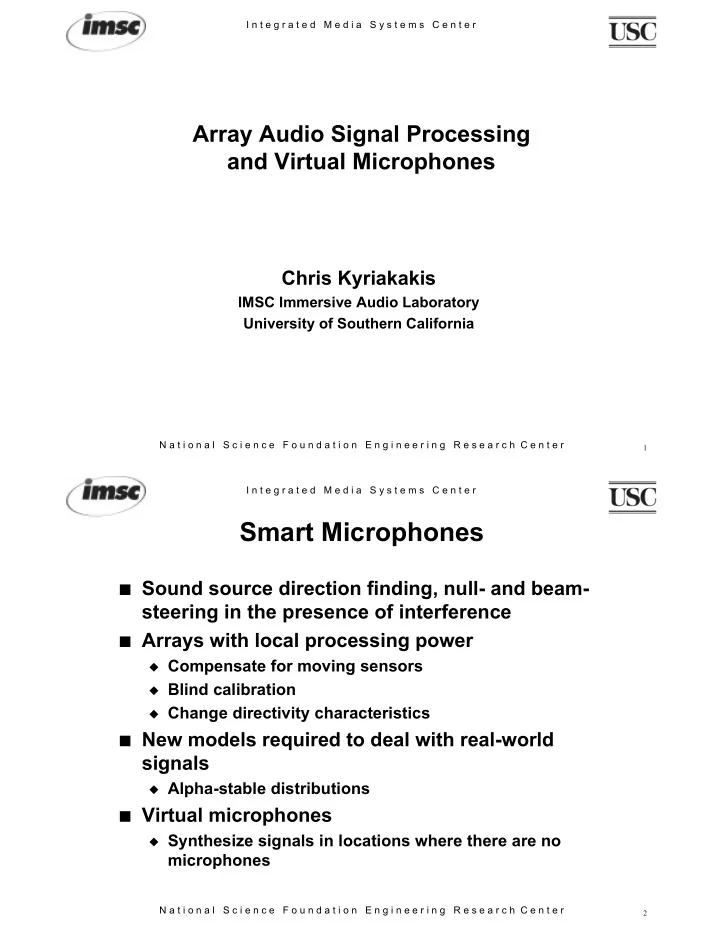
Smart Microphones n Sound source direction finding, null- and beam- - PDF document

I n t e g r a t e d M e d i a S y s t e m s C e n t e r Array Audio Signal Processing and Virtual Microphones Chris Kyriakakis IMSC Immersive Audio Laboratory University of Southern California N a t i o n a l S c i e n c e F o u n d a t i o n E n g i n e e r i n g R e s e a r c h C e n t e r 1 I n t e g r a t e d M e d i a S y s t e m s C e n t e r Smart Microphones n Sound source direction finding, null- and beam- steering in the presence of interference n Arrays with local processing power u Compensate for moving sensors u Blind calibration u Change directivity characteristics n New models required to deal with real-world signals u Alpha-stable distributions n Virtual microphones u Synthesize signals in locations where there are no microphones N a t i o n a l S c i e n c e F o u n d a t i o n E n g i n e e r i n g R e s e a r c h C e n t e r 2

I n t e g r a t e d M e d i a S y s t e m s C e n t e r Array Methods in Noisy Environments n Traditional Gaussian modeling of noise signals fails when the signals exhibit impulsive behavior n The Symmetric α -Stable ( S α S ) model, can better account for the outliers that exist in real-world signals u Example: Time Delay Estimation n In many array applications we often encounter signals that are corrupted by multiplicative noise u Traditional approach: stochastic Gaussian signal, corrupted by a Gaussian noise u Alternative: multi-dimensional Gaussian signal with LŽvy noise. N a t i o n a l S c i e n c e F o u n d a t i o n E n g i n e e r i n g R e s e a r c h C e n t e r 3 I n t e g r a t e d M e d i a S y s t e m s C e n t e r Examples of Impulsive Noise N a t i o n a l S c i e n c e F o u n d a t i o n E n g i n e e r i n g R e s e a r c h C e n t e r 4

I n t e g r a t e d M e d i a S y s t e m s C e n t e r Comparison of Gaussian and S α S models CD tray Footsteps α = 1.68 S α S α = 1.8 S α S Measured Measured Gaussian Gaussian n Real measurements in a typical room N a t i o n a l S c i e n c e F o u n d a t i o n E n g i n e e r i n g R e s e a r c h C e n t e r 5 I n t e g r a t e d M e d i a S y s t e m s C e n t e r Comparison of Gaussian and S α S models Chair Typing Gaussian α = 1.69 α = 1.44 S α S S α S Measured Gaussian Measured N a t i o n a l S c i e n c e F o u n d a t i o n E n g i n e e r i n g R e s e a r c h C e n t e r 6

I n t e g r a t e d M e d i a S y s t e m s C e n t e r New Algorithms for Time-Delay Estimation n TDE techniques based on second-order statistics fail when the noise is S α S n Alternative methods, based on Fractional Lower- Order Statistics u Fractional Lower Order Correlation Function instead of Cross Spectrum (PHAT) A R R j ω τ w = = + ε A e k 1 2 R R k A 1 2 R R 1 2 FLOS- PHAT algorithm N a t i o n a l S c i e n c e F o u n d a t i o n E n g i n e e r i n g R e s e a r c h C e n t e r 7 I n t e g r a t e d M e d i a S y s t e m s C e n t e r Performance Comparison Better 1 25 dB 0.9 6 dB 0.8 0.7 Detection score 12 dB 0.6 0.5 0.4 0.3 PHAT 0.2 FLOS-PHAT 0.1 Worse 0 α parameter 1 1.2 1.4 1.6 1.8 2 FLOS-PHAT performs better than the second-order based PHAT algorithm and adds little n computational expense N a t i o n a l S c i e n c e F o u n d a t i o n E n g i n e e r i n g R e s e a r c h C e n t e r 8

I n t e g r a t e d M e d i a S y s t e m s C e n t e r Multiple Sound Sources n κ sources and ρ sensors n Each sensor receives: κ ∑ ( ) = ( ) + ( ) x t a s t u t r r k k r , k = 1 n Array receives: ( ) + ( ) ( ) = A x t s t u t N a t i o n a l S c i e n c e F o u n d a t i o n E n g i n e e r i n g R e s e a r c h C e n t e r 9 I n t e g r a t e d M e d i a S y s t e m s C e n t e r Sub-Gaussian Signal n The Sub-Gaussian n LŽvy Distribution. signal is formed as a product of a Gaussian density with the root n This is an α -Stable distribution of a totally skewed α - with α =0.5 and completely Stable density. skewed to the right. ( β = 1) n So now the transmitted signal v(t) will be corrupted by multiplicative noise u(t) which follows the LŽvy distribution N a t i o n a l S c i e n c e F o u n d a t i o n E n g i n e e r i n g R e s e a r c h C e n t e r 10

I n t e g r a t e d M e d i a S y s t e m s C e n t e r Time Domain n Time domain of a 2 dimensional sub-Gaussian process: N a t i o n a l S c i e n c e F o u n d a t i o n E n g i n e e r i n g R e s e a r c h C e n t e r 11 I n t e g r a t e d M e d i a S y s t e m s C e n t e r Maximum Likelihood Estimator n From the Density of the sub-Gaussian distribution we can find the Maximum likelihood estimator to be: n Simulations can be made to show the effectiveness of this ML estimator N a t i o n a l S c i e n c e F o u n d a t i o n E n g i n e e r i n g R e s e a r c h C e n t e r 12

I n t e g r a t e d M e d i a S y s t e m s C e n t e r Simulations n Σ=[1 0.2 ; 0.2 1] Assuming: n 15 linearly spaced sensors n θ 1 =−0.4, θ 2 =0.6 n 2000 samples received N a t i o n a l S c i e n c e F o u n d a t i o n E n g i n e e r i n g R e s e a r c h C e n t e r 13 I n t e g r a t e d M e d i a S y s t e m s C e n t e r Virtual Microphones S 2 n Minimize appropriate cost function H 2 to find filter coefficients S 1 H 1 n LP Norms S p ( ) − ( ) = ∑ 1 F s n s n ˆ p 1 n Synthesize signal in a location where ≤ < 1 p 2 there is no microphone S H S S H S = , = 1 1 2 2 H p = = H 2 1 H p 1 2 N a t i o n a l S c i e n c e F o u n d a t i o n E n g i n e e r i n g R e s e a r c h C e n t e r 14

I n t e g r a t e d M e d i a S y s t e m s C e n t e r Audio ÒMorphingÓ ORTF Left Tymp N a t i o n a l S c i e n c e F o u n d a t i o n E n g i n e e r i n g R e s e a r c h C e n t e r 15 I n t e g r a t e d M e d i a S y s t e m s C e n t e r Virtual Mic Performance 0 −10 −20 −30 Normalized Error (dB) Normalized Error (dB) −40 −50 −60 −70 −80 −90 −100 0 2 4 6 8 10 12 14 16 18 20 Frequency (kHz) Frequency (kHz) N a t i o n a l S c i e n c e F o u n d a t i o n E n g i n e e r i n g R e s e a r c h C e n t e r 16

I n t e g r a t e d M e d i a S y s t e m s C e n t e r Multichannel Transmission Scheme n Send one channel n Synthesize remaining channels at the receiving end from a set of stored filters u Local processing can be used to generate filters 1 channel Multichannel Network Stored Filters N a t i o n a l S c i e n c e F o u n d a t i o n E n g i n e e r i n g R e s e a r c h C e n t e r 17 I n t e g r a t e d M e d i a S y s t e m s C e n t e r Conclusions n Local processing at each microphone in an array can be used to enhance performance in TDE applications and source localization in the presence of noise n Non-traditional models give better performance n Virtual microphone signals can be synthesized remotely from a single reference and a set of filters computed at the sensor N a t i o n a l S c i e n c e F o u n d a t i o n E n g i n e e r i n g R e s e a r c h C e n t e r 18