Roy L. Crole explain what inductively defined sets are; and do - - PDF document

SLIDE 1

Midlands Graduate School, University of Birmingham, April 2008 1

✬ ✫ ✩ ✪

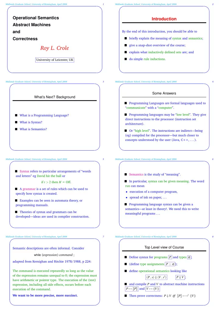
Operational Semantics Abstract Machines and Correctness

Roy L. Crole

University of Leicester, UK

Midlands Graduate School, University of Birmingham, April 2008 2

✬ ✫ ✩ ✪

Introduction

By the end of this introduction, you should be able to briefly explain the meaning of syntax and semantics; give a snap-shot overview of the course; explain what inductively defined sets are; and do simple rule inductions.

Midlands Graduate School, University of Birmingham, April 2008 3

✬ ✫ ✩ ✪

What’s Next? Background

What is a Programming Language? What is Syntax? What is Semantics?

Midlands Graduate School, University of Birmingham, April 2008 4

✬ ✫ ✩ ✪

Some Answers

Programming Languages are formal languages used to “communicate” with a “computer”. Programming languages may be “low level”. They give direct instructions to the processor (instruction set architecture). Or “high level”. The instructions are indirect—being (eg) compiled for the processor—but much closer to concepts understood by the user (Java, C++, . . . ).

Midlands Graduate School, University of Birmingham, April 2008 5

✬ ✫ ✩ ✪

Syntax refers to particular arrangements of “words and letters” eg David hit the ball or if t > 2 then H = Off. A grammar is a set of rules which can be used to specify how syntax is created. Examples can be seen in automata theory, or programming manuals. Theories of syntax and grammars can be developed—ideas are used in compiler construction.

Midlands Graduate School, University of Birmingham, April 2008 6

✬ ✫ ✩ ✪

Semantics is the study of “meaning”. In particular, syntax can be given meaning. The word run can mean

• execution of a computer program,
• spread of ink on paper, . . .

Programming language syntax can be given a semantics—at least in theory!. We need this to write meaningful programs . . .

Midlands Graduate School, University of Birmingham, April 2008 7

✬ ✫ ✩ ✪

Semantic descriptions are often informal. Consider

while (expression) command ;

adapted from Kernighan and Ritchie 1978/1988, p 224: The command is executed repeatedly so long as the value

• f the expression remains unequal to 0; the expression must

have arithmetic or pointer type. The execution of the (test) expression, including all side effects, occurs before each execution of the command. We want to be more precise, more succinct.

Midlands Graduate School, University of Birmingham, April 2008 8

✬ ✫ ✩ ✪

Top Level view of Course

Define syntax for programs P and types σ ; (define type assignments P :: σ ); define operational semantics looking like (P, s) ⇓ (V , s′) P ⇓ V ; and compile P and V to abstract machine instructions P → [[P]] and V → (|V|) Then prove correctness: P ⇓ V iff [[P]] − →t (|V|)

SLIDE 2

Midlands Graduate School, University of Birmingham, April 2008 9

✬ ✫ ✩ ✪

What’s Next? Inductively Defined Sets

Specify inductively defined sets; programs, types etc will be defined this way. BNF grammars are a form of inductive definition; abstract syntax trees are also defined inductively. Define Rule Induction; properties of programs will be proved using this. It is important.

Midlands Graduate School, University of Birmingham, April 2008 10

✬ ✫ ✩ ✪

Example Inductive Definition

Let Var be a set of propositional variables. Then the set Prpn

• f propositions of propositional logic is inductively defined

by the rules [P ∈ Var] (A) P φ ψ (∧) φ∧ψ φ ψ (∨) φ∨ψ φ ψ (→) φ → ψ φ (¬) ¬φ Each proposition is created by a deduction . . .

Midlands Graduate School, University of Birmingham, April 2008 11

✬ ✫ ✩ ✪

Inductively Defined Sets in General

Given a set of rules, a deduction is a finite tree such that − each leaf node label c occurs as a base rule (∅,c) ∈ R − for any non-leaf node label c, if H is the set of children of c then (H,c) ∈ R is an inductive rule. The set I inductively defined by R consists of those elements e which have a deduction with root node e. One may prove ∀e ∈ I. φ(e) for a property φ(e) by rule

• induction. See the notes . . .

Midlands Graduate School, University of Birmingham, April 2008 12

✬ ✫ ✩ ✪

Example of Rule Induction

Consider the set of trees T defined inductively by [n ∈ Z] n T1 T2 +(T1,T2) Let L(T) be the number of leaves in T, and N(T) be the number of +-nodes of T. We prove (see board) ∀T ∈ T . L(T) = N(T)+1 where the functions L,N:T → N are defined recursively by

• L(n) = 1 and L(+(T1,T2)) = L(T1)+L(T2)
• N(n) = 0 and N(+(T1,T2)) = N(T1)+N(T2)+1

Midlands Graduate School, University of Birmingham, April 2008 13

✬ ✫ ✩ ✪

Chapter 1

By the end of this chapter, you should be able to describe the programs (syntax) of a simple imperative language called IMP; give a type system to IMP and derive types; explain the idea of evaluation relations; derive example evaluations.

Midlands Graduate School, University of Birmingham, April 2008 14

✬ ✫ ✩ ✪

What’s Next? Types and Expressions

We define the types and expressions of IMP. We give an inductive definition of a formal type system.

Midlands Graduate School, University of Birmingham, April 2008 15

✬ ✫ ✩ ✪

Program Expressions and Types for IMP

The program expressions are given (inductively) by P ::= c constant | l memory location | P iop P′ integer operator | P bop P′ boolean operator | l:=P′ assignment | P ; P′ sequencing | if P then P′ else P′′ conditional | while P do P′ while loop

Midlands Graduate School, University of Birmingham, April 2008 16

✬ ✫ ✩ ✪

The types of the language IMP are given by the grammar σ ::= int | bool | cmd A location environment L is a finite set of (location, type) pairs, with type being just int or bool:

L = l1 :: int,...,ln :: int, ln+1 :: bool,...,lm :: bool

Given L, then any P whose locations all appear in L can (sometimes) be assigned a type; we write P :: σ to indicate this, and define such type assignments inductively.

SLIDE 3

Midlands Graduate School, University of Birmingham, April 2008 17

✬ ✫ ✩ ✪

[any n ∈ Z] n :: int T :: bool F :: bool [l :: int ∈ L] l :: int P1 :: int P2 :: int [ bop ∈ BOpr] P1 bop P2 :: bool skip :: cmd l :: σ P :: σ l:=P :: cmd P1 :: bool P2 :: cmd P3 :: cmd if P1 then P2 else P3 :: cmd P1 :: bool P2 :: cmd while P1 do P2 :: cmd

Midlands Graduate School, University of Birmingham, April 2008 18

✬ ✫ ✩ ✪

Example: Deduction of a Type Assignment

l :: int 5 :: int l ≥ 5 :: bool

D2 D3 D4

l:=l−1 ; l′ :=l′ ∗l :: cmd if l ≥ 5 then l′ :=1 else (l:=l+1 ; l′ :=l′ ∗l) :: cmd

Midlands Graduate School, University of Birmingham, April 2008 19

✬ ✫ ✩ ✪

What’s Next? An Evaluation Relation

We define a notion of state. We define an evaluation relation for IMP. We look at an example.

Midlands Graduate School, University of Birmingham, April 2008 20

✬ ✫ ✩ ✪

States

A state s is a finite partial function Loc → Z∪B. For example s = l1 → 4,l2 → T,l3 → 21 There is a state denoted by s{l→c} : Loc → Z∪B which is the partial function (s{l→c})(l′) def =    c if l′ = l s(l′)

• therwise

We say that state s is updated at l by c.

Midlands Graduate School, University of Birmingham, April 2008 21

✬ ✫ ✩ ✪

An Evaluation Relation

Consider the following evaluation relationship ( l′ :=T ; l:=4+1 , ) ⇓ ( skip , l′ → T,l → 5 ) The idea is Starting program ⇓ final result We describe an operational semantics which has assertions which look like (P, s) ⇓ (c, s) and (P, s1) ⇓ (skip, s2)

Midlands Graduate School, University of Birmingham, April 2008 22

✬ ✫ ✩ ✪

[ provided l ∈ domain of s]⇓LOC (l, s) ⇓ (s(l), s) (P1 , s) ⇓ (n1 , s) (P2 , s) ⇓ (n2 , s) ⇓OP (P1 op P2 , s) ⇓ (n1 op n2 , s) (P, s) ⇓ (c, s) ⇓ASS (l:=P, s) ⇓ (skip, s{l→c}) (P1 , s1) ⇓ (skip, s2) (P2 , s2) ⇓ (skip, s3) ⇓SEQ (P1 ; P2 , s1) ⇓ (skip, s3)

Midlands Graduate School, University of Birmingham, April 2008 23

✬ ✫ ✩ ✪

(P, s1) ⇓ (F, s1) (P2 , s1) ⇓ (skip, s2) ⇓COND2 (if P then P1 else P2 , s1) ⇓ (skip, s2) (P1 , s1) ⇓ (T , s1) (P2 , s1) ⇓ (skip, s2) (while P1 do P2 , s2) ⇓ (skip, s3) (while P1 do P2 , s1) ⇓ (skip, s3) (P1 , s) ⇓ (F, s) ⇓LOOP2 (while P1 do P2 , s) ⇓ (skip, s)

Midlands Graduate School, University of Birmingham, April 2008 24

✬ ✫ ✩ ✪

Example Evaluations

We derive deductions for ((3+2)∗6, s) ⇓ (30, s) and (while l = 1 do l:=l−1, l → 1) ⇓ (skip, l → 0)

SLIDE 4

Midlands Graduate School, University of Birmingham, April 2008 25

✬ ✫ ✩ ✪

Chapter 2

By the end of this chapter you should be able to describe the “compiled” CSS machine, which executes compiled IMP programs; show how to compile to CSS instruction sequences; give some example executions.

Midlands Graduate School, University of Birmingham, April 2008 26

✬ ✫ ✩ ✪

Motivating the CSS Machine

An operational semantics gives a useful model of IMP—we seek a more direct, “computational” method for evaluating

• configurations. If P ⇓e V, how do we “mechanically

produce” V from P? P ≡ P0 → P1 → P2 → ... → Pn ≡ V “Mechanically produce” can be made precise using a relation P − → P′ defined by rules with no hypotheses. n+m − → m+n

Midlands Graduate School, University of Birmingham, April 2008 27

✬ ✫ ✩ ✪

P0 → P1 → P2 → P3 → P4 ... → V Re-Write Rules (Abstract Machine)

deduction tree

P ⇓e

✛ ✲

V Evaluation Semantics

Midlands Graduate School, University of Birmingham, April 2008 28

✬ ✫ ✩ ✪

An Example

Let s(l) = 6. Execute 10−l on the CSS machine. First, compile the program. [[10−l]] =

FETCH(l) : PUSH(10) : OP(−)

Then

FETCH(l) : PUSH(10) : OP(−)

− s − → PUSH(10) : OP(−) 6 s − → OP(−) 10 : 6 s − → − 4 s

Midlands Graduate School, University of Birmingham, April 2008 29

✬ ✫ ✩ ✪

Defining the CSS Machine

A CSS code C is a list: C ::= − | ins : C ins ::=

PUSH(c) | FETCH(l) | OP(op) | SKIP

| STO(l) | BR(C,C) | LOOP(C,C) The objects ins are CSS instructions. We will overload : to denote append; and write ξ for ξ : − (ditto below). A stack S is produced by the grammar S ::= − | c : S

Midlands Graduate School, University of Birmingham, April 2008 30

✬ ✫ ✩ ✪

A CSS configuration is a triple (C,S,s). A CSS re-write takes the form (C1, S1 , s1 ) − → (C2 , S2 , s2 ) and re-writes are specified inductively by rules with no hypotheses (such rules are often called axioms) R (C1, S1 , s1 ) − → (C2, S2 , s2 ) Note that the CSS re-writes are deterministic.

Midlands Graduate School, University of Birmingham, April 2008 31

✬ ✫ ✩ ✪ PUSH(c) : C

S s − → C c : σ s

FETCH(l) : C

S s − → C s(l) : S s

OP( op ) : C

n1 : n2 : S s − → C n1 op n2 : S s

STO(l) : C

c : S s − → C S s{l→c}

BR(C1,C2) : C

F : S s − → C2 : C S s

LOOP(C1,C2) : C

S s − → C1 : BR(C2 : LOOP(C1,C2),SKIP) : C S s

Midlands Graduate School, University of Birmingham, April 2008 32

✬ ✫ ✩ ✪

[[c]]

def

=

PUSH(c)

[[l]]

def

=

FETCH(l)

[[P1 op P2]]

def

= [[P2]] : [[P1]] : OP(op) [[l:=P]]

def

= [[P]] : STO(l) [[skip]]

def

=

SKIP

[[P1 ; P2]]

def

= [[P1]] : [[P2]] [[if P then P1 else P2]]

def

= [[P]] : BR([[P1]],[[P2]]) [[while P1 do P2]]

def

=

LOOP([[P1]],[[P2]])

SLIDE 5

Midlands Graduate School, University of Birmingham, April 2008 33

✬ ✫ ✩ ✪

Chapter 3

By the end of this chapter you should be able to describe the “interpreted” CSS machine, which executes IMP programs; explain the outline of a proof of correctness; explain some of the results required for establishing correctness, and the proofs of these results.

Midlands Graduate School, University of Birmingham, April 2008 34

✬ ✫ ✩ ✪

Architecture of the Machine

A CSS code C is a list of instructions which is produced by the following grammars: C ::= − | ins : C ins ::= P | op | STO(l) | BR(P1,P2) We will overload : to denote append; and write ξ for ξ : − (ditto below). A stack S is produced by the grammar S ::= − | c : S

Midlands Graduate School, University of Birmingham, April 2008 35

✬ ✫ ✩ ✪

n : C S s − → C n : σ s P1 op P2 : C S s − → P2 : P1 : op : C S s

• p : C

n1 : n2 : S s − → C n1 op n2 : S s l:=P : C S s − → P : STO(l) : C S s

STO(l) : C

n : S s − → C S s{l→n} while P1 do P2 : C S s − → P1 : BR((P2 ; while P1 do P2),skip) : C S s

Midlands Graduate School, University of Birmingham, April 2008 36

✬ ✫ ✩ ✪

A Correctness Theorem

For all n ∈ Z, b ∈ B, P1 :: int, P2 :: bool, P3 :: cmd and s,s1,s2 ∈ States we have (P1 , s) ⇓ (n, s) iff P1 − s − →t − n s (P2 , s) ⇓ (b, s) iff P2 − s − →t − b s (P3 , s1) ⇓ (skip, s2) iff P3 − s1 − →t − − s2 where − →t denotes the transitive closure of − →.

Midlands Graduate School, University of Birmingham, April 2008 37

✬ ✫ ✩ ✪

Proof Method

= ⇒onlyif by Rule Induction for ⇓. ⇐ =if by Mathematical Induction on k. Recall κ − →t κ′ iff (∃ k ≥ 1)(κ − →k κ′), where for k ≥ 1, κ − →k κ′ means that (∀1 ≤ i ≤ k)(∃κi)(κ − → κ1 − → ... − → κk = κ′) Then note if the ✷ are configurations with ξ parameters (∀ξ)( (∃k)(✷ − →k ✷) implies ✷ ⇓ ✷ ) ≡ (∀k)(∀ξ) (✷ − →k ✷ implies ✷ ⇓ ✷)

• φ(k)

Midlands Graduate School, University of Birmingham, April 2008 38

✬ ✫ ✩ ✪

Code and Stack Extension

For all k ∈ N, and for all appropriate codes, stacks and states, C1 S1 s1 − →k C2 S2 s2 implies C1 : C3 S1 : S3 s1 − →k C2 : C3 S2 : S3 s2 where − →0 is reflexive closure of − →.

Midlands Graduate School, University of Birmingham, April 2008 39

✬ ✫ ✩ ✪

Code Splitting

For all k ∈ N, and for all appropriate codes, stacks and states, if C1 : C2 S s − →k − S′′ s′′ then there is a stack and state S′ and s′, and k1,k2 ∈ N for which C1 S s − →k1 − S′ s′ C2 S′ s′ − →k2 − S′′ s′′ where k1 +k2 = k.

Midlands Graduate School, University of Birmingham, April 2008 40

✬ ✫ ✩ ✪

Typing and Termination Yields Values

For all k ∈ N, and for all appropriate codes, stacks, states, P :: int and P S s − →k − S′ s′ implies s = s′ and S′ = n : S some n ∈ Z and P − s − →k − n s and similarly for Booleans.

SLIDE 6

Midlands Graduate School, University of Birmingham, April 2008 41

✬ ✫ ✩ ✪

Proving the Theorem

(= ⇒onlyif ): Rule Induction for ⇓ (Case ⇓ OP1): The inductive hypotheses are P1 − s − →t − n1 s P2 − s − →t − n2 s Then P1 op P2 − s − → P2 : P1 : op − s − →t P1 : op n2 s ≡ P1 : op n2 s − →t

• p

n1 : n2 s − → − n1 op n2 s

Midlands Graduate School, University of Birmingham, April 2008 42

✬ ✫ ✩ ✪

(⇐ =if): We prove by induction for all k, for all P :: int,n,s, P − s − →k − n s implies (P, s) ⇓ (n, s)

• φ(k)

(Proof of ∀k0 ∈ N, φ(k)k≤k0 implies φ(k0 +1)): Suppose that for some arbitrary k0, P :: int, n and s P − s − →k0+1 − n s (∗) and then we prove (P, s) ⇓ (n, s) by considering cases on P.

Midlands Graduate School, University of Birmingham, April 2008 43

✬ ✫ ✩ ✪

(Case P is P1 op P2): Suppose that P1 op P2 − s − →k0+1 − n s and so P2 : P1 : op − s − →k0 − n s . Using splitting and termination we have, noting P2 :: int, that P2 − s − →k1 − n2 s P1 : op n2 s − →k2 − n s where k1 +k2 = k0,

Midlands Graduate School, University of Birmingham, April 2008 44

✬ ✫ ✩ ✪

and repeating for the latter re-write we get P1 n2 s − →k21 − n1 : n2 s

• p

n1 : n2 s − →k22 − n s (1) where k21 +k22 = k2. So as k1 ≤ k0, by induction we deduce that (P2 , s) ⇓ (n2 , s), and from termination that P1 − s − →k21 − n1 s . Also, as k21 ≤ k0, we have inductively that (P1 , s) ⇓ (n1 , s) and hence (P1 op P2 , s) ⇓ (n1 op n2 , s). But from determinism and (1) we see that n1 op n2 = n and we are done.

Midlands Graduate School, University of Birmingham, April 2008 45

✬ ✫ ✩ ✪

Chapter 4

By the end of this chapter you should be able to describe the expressions and type system of a language with higher order functions; explain how to write simple programs; specify an eager evaluation relation; prove properties such as determinism.

Midlands Graduate School, University of Birmingham, April 2008 46

✬ ✫ ✩ ✪

What’s Next? Expressions and Types for FUN

Define the expression syntax and type system.

Midlands Graduate School, University of Birmingham, April 2008 47

✬ ✫ ✩ ✪

Examples of FUN Declarations

g :: Int -> Int -> Int g x y = x+y l1 :: [Int] l1 = 5:(6:(8:(4:(nil)))) h :: Int h = hd (5:6:8:4:nil) length :: [Bool] -> Int length l = if elist(l) then 0 else (1 + length t)

Midlands Graduate School, University of Birmingham, April 2008 48

✬ ✫ ✩ ✪

FUN Types

The types of FUNe are σ ::= int | bool | σ → σ | [σ] We shall write σ1 → σ2 → σ3 → ... → σn → σ for σ1 → (σ2 → (σ3 → (... → (σn → σ)...))). Thus for example σ1 → σ2 → σ3 means σ1 → (σ2 → σ3).

SLIDE 7

Midlands Graduate School, University of Birmingham, April 2008 49

✬ ✫ ✩ ✪

FUN Expressions

The expressions are

E ::= x variables | c constants | K constant identifier | F function identifier | E1 E2 function application | tl(E) tail of list | E1 : E2 cons for lists | elist(E) Boolean test for empty list Bracketing conventions apply . . .

Midlands Graduate School, University of Birmingham, April 2008 50

✬ ✫ ✩ ✪

What’s Next? A Formal FUN Type System

Show how to declare the types of variables and identifiers. Give some examples. Define a type assignment system.

Midlands Graduate School, University of Birmingham, April 2008 51

✬ ✫ ✩ ✪

Contexts (Variable Environments)

When we write a FUN program, we shall declare the types of variables, for example x :: int,y :: bool,z :: bool A context, variables assumed distinct, takes the form Γ = x1 :: σ1,...,xn :: σn.

Midlands Graduate School, University of Birmingham, April 2008 52

✬ ✫ ✩ ✪

Identifier Environments

When we write a FUN program, we want to declare the types of constants and functions. A simple example of an identifier environment is K :: bool, map :: (int → int) → [int] → [int], suc :: int → int An identifier type looks like σ1 → σ2 → σ3 → ... → σa → σ where a ≥ 0 and σ is NOT a function type. An identifier environment looks like

I = I1 :: ι1,...,Im :: ιm.

Midlands Graduate School, University of Birmingham, April 2008 53

✬ ✫ ✩ ✪

Example Type Assignments

With the previous identifier environment x :: int,y :: int,z :: int ⊢ mapsuc(x : y : z : nilint) :: [int] We have ∅ ⊢ if T then hd(2 : nilint) else hd(4 : 6 : nilint) :: int

Midlands Graduate School, University of Birmingham, April 2008 54

✬ ✫ ✩ ✪

Inductively Defining Type Assignments

Start with an identifier environment I and a context Γ. Then ( where x :: σ ∈ Γ) :: VAR Γ ⊢ x :: σ :: INT Γ ⊢ n :: int Γ ⊢ E1 :: int Γ ⊢ E2 :: int :: OP1 Γ ⊢ E1 iop E2 :: int

Midlands Graduate School, University of Birmingham, April 2008 55

✬ ✫ ✩ ✪

Γ ⊢ E1 :: σ2 → σ1 Γ ⊢ E2 :: σ2 :: AP Γ ⊢ E1 E2 :: σ1 ( where I :: ι ∈ I) :: IDR Γ ⊢ I :: ι :: NIL Γ ⊢ nilσ :: [σ] Γ ⊢ E1 :: σ Γ ⊢ E2 :: [σ] :: CONS Γ ⊢ E1 : E2 :: [σ]

Midlands Graduate School, University of Birmingham, April 2008 56

✬ ✫ ✩ ✪

What’s Next? Function Declarations and Programs

Show how to code up functions. Define what makes up a FUN program. Give some examples.

SLIDE 8

Midlands Graduate School, University of Birmingham, April 2008 57

✬ ✫ ✩ ✪

Introducing Function Declarations

To declare plus can write plus x y = x+y. To declare fac fac x = if x == 1 then 1 else x∗fac(x−1) And to declare that true denotes T we write true = T. In FUNe , can specify (recursive) declarations K = E Fx = E′ G x y = E′′ ...

Midlands Graduate School, University of Birmingham, April 2008 58

✬ ✫ ✩ ✪

An Example Declaration

Let I = I1 :: [int] → int → int,I2 :: int → int,I3 :: bool. Then an example of an identifier declaration decI is I1 l y = hd(tl(tl(l)))+I2 y

def

= EI1 I2x = x∗x

def

= EI2 I3 = T

def

= EI3 I4 u v w = u+v+w

def

= EI4

Midlands Graduate School, University of Birmingham, April 2008 59

✬ ✫ ✩ ✪

An Example Program

Let I = F :: int → int → int,K :: int. Then an identifier declaration decI is F x y = x+7−y

def

= EF K = 10 An example of a program is decI in F 8 1 ≤ K . Note that ∅ ⊢ F 8 1 ≤ K :: bool and x :: int,y :: int

• ΓF

⊢ x+7−y :: int

• σF

and ∅ ⊢ K :: int

Midlands Graduate School, University of Birmingham, April 2008 60

✬ ✫ ✩ ✪

Defining Programs

A program in FUNe is a judgement of the form decI in P where decI is a given identifier declaration and the program expression P satisfies a type assignment of the form ∅ ⊢ P :: σ (written P :: σ) and ∀ F x = EF ∈ decI ΓF ⊢ EF :: σF

Midlands Graduate School, University of Birmingham, April 2008 61

✬ ✫ ✩ ✪

What’s Next? Values and the Evaluation Relation

Look at the notion of evaluation order. Define values, which are the results of eager program executions. Define an eager evaluation semantics: P ⇓e V. Give some examples.

Midlands Graduate School, University of Birmingham, April 2008 62

✬ ✫ ✩ ✪

Evaluation Orders

The operational semantics of FUNe says when a program P evaluates to a value V. It is like the IMP evaluation semantics. Write this in general as P ⇓e V, and examples are 3+4+10 ⇓e 17 hd(2 : nilint) ⇓e 2

Midlands Graduate School, University of Birmingham, April 2008 63

✬ ✫ ✩ ✪

Let F x y = x+y. We would expect F (2∗3) (4∗5) ⇓e 26. We could

• evaluate 2∗3 to get value 6 yielding F 6 (4∗5),
• then evaluate 4∗5 to get value 20 yielding F 6 20.

We then call the function to get 6+20, which evaluates to

• 26. This is call-by-value or eager evaluation.

Or the function could be called first yielding (2∗3)+(4∗5) and then we continue to get 6+(4∗5) and 6+20 and 26. This is called call-by-name or lazy evaluation.

Midlands Graduate School, University of Birmingham, April 2008 64

✬ ✫ ✩ ✪

Defining and Explaining (Eager) Values

Let decI be an identifier declaration, with typical typing F :: σ1 → σ2 → σ3 → ... → σa → σ Informally a is the maximum number of inputs taken by F. A value expression is any expression V produced by V ::= c | nilσ | F V | V : V where V abbreviates V1 V2 ... Vk−1 Vk and 0 ≤ k < a. Note also that k is strictly less than a, and that if a = 1 then F V denotes F.

SLIDE 9

Midlands Graduate School, University of Birmingham, April 2008 65

✬ ✫ ✩ ✪

A value is any value expression for which decI in V is a valid FUNe program. Suppose that F :: int → int → int → int and that P1 ⇓e 2 and P2 ⇓e 5 and P3 ⇓e 7 with Pi not values. Then P V F F P1 F 2 F 2 P2 F 2 5 P V F 2 5 P3 F 2 5 7 14 F P1 P2 P3 14

Midlands Graduate School, University of Birmingham, April 2008 66

✬ ✫ ✩ ✪

The Evaluation Relation

⇓eVAL V ⇓e V P1 ⇓e m P2 ⇓e n ⇓eOP P1 op P2 ⇓e m op n P1 ⇓e T P2 ⇓e V ⇓eCOND1 if P1 then P2 else P3 ⇓e V

Midlands Graduate School, University of Birmingham, April 2008 67

✬ ✫ ✩ ✪    P1 ⇓e F V P2 ⇓e V2 F V V2 ⇓e V where either P1 or P2 is not a value ⇓eAP P1 P2 ⇓e V EF[V1,...,Va/x1,...,xa] ⇓e V [F x = EF declared in decI ] ⇓eFID FV1 ...Va ⇓e V EK ⇓e V [K = EK declared in decI ] ⇓eCID K ⇓e V

Midlands Graduate School, University of Birmingham, April 2008 68

✬ ✫ ✩ ✪ P ⇓e V : V′ ⇓eHD hd(P) ⇓e V P ⇓e V : V′ ⇓eTL tl(P) ⇓e V′ P1 ⇓e V P2 ⇓e V′ ⇓eCONS P1 : P2 ⇓e V : V′ P ⇓e nilσ ⇓eELIST1 elist(P) ⇓e T P ⇓e V : V′ ⇓eELIST2 elist(P) ⇓e F

Midlands Graduate School, University of Birmingham, April 2008 69

✬ ✫ ✩ ✪

Examples of Evaluations

Suppose that decI is G x = x∗2 K = 3

VAL

G ⇓e G

VAL

3 ⇓e 3

CID

K ⇓e 3

VAL

3 ⇓e 3

VAL

2 ⇓e 2

OP

(x∗2)[3/x] = 3∗2 ⇓e 6

FID

G 3 ⇓e 6

AP

G K ⇓e 6

Midlands Graduate School, University of Birmingham, April 2008 70

✬ ✫ ✩ ✪

We can prove that F 2 3 (4+1) ⇓e 10 where F x y z = x+y+z as follows: ⇓e VAL F 2 3 ⇓e F 2 3 4 ⇓e 4 1 ⇓e 1 4+1 ⇓e 5 T ⇓e AP F 2 3 (4+1) ⇓e 10

Midlands Graduate School, University of Birmingham, April 2008 71

✬ ✫ ✩ ✪

where T is the tree 2 ⇓e 2 3 ⇓e 3 2+3 ⇓e 5 5 ⇓e 5 2+3+5 ⇓e 10 = = = = = = = = = = = = = = = = = = = = = = = = = = (x+y+z)[2,3,5/x,y,z] ⇓e 10 ⇓e FID F 2 3 5 ⇓e 10

Midlands Graduate School, University of Birmingham, April 2008 72

✬ ✫ ✩ ✪

What’s Next? FUN Properties of Eager Evaluation

Explain and define determinism. Explain and define subject reduction, that is, preservation of types during program execution.

SLIDE 10

Midlands Graduate School, University of Birmingham, April 2008 73

✬ ✫ ✩ ✪

Properties of FUN

The evaluation relation for FUNe is deterministic. More precisely, for all P, V1 and V2, if P ⇓e V1 and P ⇓e V2 then V1 = V2. (Thus ⇓e is a partial function.) Evaluating a program decI in P does not alter its

• type. More precisely,

(∅ ⊢ P :: σ and P ⇓e V) implies ∅ ⊢ V :: σ for any P, V, σ and decI. The conservation of type during program evaluation is called subject reduction.

Midlands Graduate School, University of Birmingham, April 2008 74

✬ ✫ ✩ ✪

Chapter 5

By the end of this chapter you should be able to describe the SECD machine, which executes compiled FUNe programs; here the expressions Exp are defined by E ::= x | n | F | E E; show how to compile to SECD instruction sequences; write down example executions.

Midlands Graduate School, University of Birmingham, April 2008 75

✬ ✫ ✩ ✪

Architecture of the Machine

The SECD machine consists of rules for transforming SECD configurations (S,E,C,D). The non-empty stack S is generated by S ::= n ↑ | Sl ...S1 cloF ↑ Each node occurs at a level ≥ 1. A stack S has a height the maximum level of any cloF, or 0

• therwize.

Midlands Graduate School, University of Birmingham, April 2008 76

✬ ✫ ✩ ✪

If the (unique) left-most closure node cloF at level α exists, call it the α-prescribed node, and write α S. For any stack α S of height ≥ 1 there is a sub-stack S′

• f shape

Sl ... S1 cloF ↑

Midlands Graduate School, University of Birmingham, April 2008 77

✬ ✫ ✩ ✪

Given any other stack Sl+1 there is a stack S′′ Sl+1 Sl ... S1 cloF ↑ Write Sl+1 ⊕S for S with S′ replaced by S′′.

Midlands Graduate School, University of Birmingham, April 2008 78

✬ ✫ ✩ ✪

The environment E takes the form x1 =?S1 : ... : xn =?Sn. The value of each ? is determined by the form of an Si. If Si is n ↑ then ? is 0; if Si is cloF ↑ then ? is 1; in any

• ther case, ? is Av1.

Midlands Graduate School, University of Birmingham, April 2008 79

✬ ✫ ✩ ✪

A SECD code C is a list which is produced by the following grammars: ins ::= x | n | F | APP C ::= − | ins : C A typical dump looks like (S1,E1,C1,(S2,E2,C2,...(Sn,En,Cn,−)...)) We will overload : to denote append; and write ξ for ξ : −.

Midlands Graduate School, University of Birmingham, April 2008 80

✬ ✫ ✩ ✪

We define a compilation function [[−]]:Exp → SECDcodes which takes an SECD expression and turns it into code. [[x]] def = x [[n]] def = n [[F]] def = F [[E1 E2]] def = [[E1]] : [[E2]] : APP

SLIDE 11

Midlands Graduate School, University of Birmingham, April 2008 81

✬ ✫ ✩ ✪

There is a representation of program values as stacks, given by (|n|) def = n ↑

• (|F V1 ...Vk|) def

= (|Vk|) ... (|V1|) cloF ↑ = (|Vk|)⊕...⊕(|V1|)⊕ cloF ↑ Recall k < a with a the arity of F.

Midlands Graduate School, University of Birmingham, April 2008 82

✬ ✫ ✩ ✪

The Re-writes

A number is pushed onto the stack (the initial stack can be

• f any status):

S [Av]α S E E C n : C D D

num

− → S α n ↑ ⊕S E E C C D D

Midlands Graduate School, University of Birmingham, April 2008 83

✬ ✫ ✩ ✪

A function is pushed onto the stack (the initial stack can be

• f any status):

S [Av]α S E E C F : C D D

fn

− → S α+1 cloF ↑ ⊕S E E C C D D

Midlands Graduate School, University of Birmingham, April 2008 84

✬ ✫ ✩ ✪

A variable’s value is pushed onto the stack, provided that the environment E contains x = ?T ≡ [Av]δ T (where δ is 0 or 1). Note that by definition, the status of T determines the status

• f the re-written stack:

S [Av]α S E E C x : C D D

var

− → S [Av]δ+α T ⊕S E E C C D D

Midlands Graduate School, University of Birmingham, April 2008 85

✬ ✫ ✩ ✪

An APP command creates an application value, type 0:

S α Sk ...S1 cloF ↑ ⊕S E E C APP : C D D

cav0

− → S

Avα

Sk ...S1 cloF ↑ ⊕S E E C C D D

Midlands Graduate School, University of Birmingham, April 2008 86

✬ ✫ ✩ ✪

An APP command creates an application value, type 1:

S α cloH ↑ Sk−1 ...S1 cloF ↑ ⊕S E E C APP : C D D

cav1

− → S

Avα−1

cloH ↑ Sk−1 ...S1 cloF ↑ ⊕S E E C C D D

Midlands Graduate School, University of Birmingham, April 2008 87

✬ ✫ ✩ ✪

An APP command produces an application value from an application value:

S

Avα

Sk ...S1 cloF ↑ S′

k′−1 ...S′ 1

cloG ↑ ⊕S E E C APP : C D D

avtav

− → S

Avα−1

Sk ...S1 cloF ↑ S′

k′−1 ...S′ 1

cloG ↑ ⊕S E E C C D D

Midlands Graduate School, University of Birmingham, April 2008 88

✬ ✫ ✩ ✪

An APP command calls a function, type 0:

S α Sa ...S1 cloF ↑ ⊕S E E C APP : C D D

call0

− → S − E xa = ?Sa : ... : x1 = ?S1 : E C [[EF]] D (α−1 S,E,C,D)

SLIDE 12

Midlands Graduate School, University of Birmingham, April 2008 89

✬ ✫ ✩ ✪

An APP command calls a function, type 1:

S α cloH ↑ Sa−1 ...S1 cloF ↑ ⊕S E E C APP : C D D

call1

− → S − E xa =?Sa : ... : x1 =?S1 : E C [[EF]] D (α−2 S,E,C,D)

Midlands Graduate School, University of Birmingham, April 2008 90

✬ ✫ ✩ ✪

An APP command calls a function, type 2:

S

Avα

Sk ...S1 cloF ↑ S′

a−1 ...S′ 1

cloG ↑ ⊕S E E C APP : C D D

call2

− → S − E xa =?S′

a : ... : x1 =?S′ 1 : E

C [[EG]] D (α−2 S,E,C,D)

Midlands Graduate School, University of Birmingham, April 2008 91

✬ ✫ ✩ ✪

Restore, where the final status is determined by the initial status: S [Av]β T E E′ C − D (α S,E,C,D)

res

− → S [Av]α+β T ⊕S E E C C D D

Midlands Graduate School, University of Birmingham, April 2008 92

✬ ✫ ✩ ✪

Suppose that K, N and MN are functions which are also values, and that F x y = x L u v = u I a b = b H z = L (M N) z Then (F (H 4)) (I 2 K) ⇓e M N. Note that [[(F (H 4)) (I 2 K)]] = (11. def = F) : H : 4 : APP : APP : I : 2 : APP : K : APP : (APP def = 1.) and [[L (M N) z]] def = 7. def = L : M : N : APP : APP : z : APP def = 1.

Midlands Graduate School, University of Birmingham, April 2008 93

✬ ✫ ✩ ✪

S − E − C 11. D −

num/fn

− →

3

S 2 4 ↑ cloH ↑ cloF ↑ E − C

• 8. ≡ APP : 7.

D −

Midlands Graduate School, University of Birmingham, April 2008 94

✬ ✫ ✩ ✪

call0

− → S − E E′ def = z = 0 4 ↑ C [[L (M N) z]] D ξ def = (1 cloF ↑ ,−,7.,−)

fn

− →

3

S 3 cloN ↑ cloM ↑ cloL ↑ E E′ C 4. D ξ

Midlands Graduate School, University of Birmingham, April 2008 95

✬ ✫ ✩ ✪

cav1

− → S

Av2

cloN ↑ cloM ↑ cloL ↑ E E′ C 3. D ξ

avtav

− → S

Av1

cloN ↑ cloM ↑ cloL ↑ E E′ C 2. D ξ

Midlands Graduate School, University of Birmingham, April 2008 96

✬ ✫ ✩ ✪

Chapter 6

By the end of this chapter you should be able to explain the outline of a proof of correctness; explain some of the results required for establishing correctness, and the proofs of these results.

SLIDE 13

Midlands Graduate School, University of Birmingham, April 2008 97

✬ ✫ ✩ ✪

A Correctness Theorem

For all programs decI in P for which ∅ ⊢ P :: σ we have P ⇓e V iff S − E − C [[P]] D − − →t S (|V|) E − C − D −

Midlands Graduate School, University of Birmingham, April 2008 98

✬ ✫ ✩ ✪

Code and Stack Extension

For any stacks, environments, codes, and dumps, if C1 is non-empty

M def = S S1 E E C C1 D D − →k S S2 E E C C2 D D

def

= M′ implies M def = S S1 ⊕S3 E E C C1 : C3 D D − →k S S2 ⊕S3 E E C C2 : C3 D D

def

= M′

Midlands Graduate School, University of Birmingham, April 2008 99

✬ ✫ ✩ ✪

Need to prove “lemma plus”: if D ≡ (S′,E′,C′,D′) we can also similarly arbitrarily extend any of the stacks and codes in D (say to D). We use induction on k. Suppose lemma plus is true ∀k ≤ k0. Must prove we can extend any re-write M − →k0+1 M′ to M − →k0+1 M′. By determinism, we have M − →1 M′′ − →k0 M′. If no function call during M − →1 M′′, trivial to extend to get M − →1 M′′. And by induction, M′′ − →k0 M′.

Midlands Graduate School, University of Birmingham, April 2008 100

✬ ✫ ✩ ✪

If there is a function call, there are k1 and k2 such that M def = S T ⊕S E E C APP : C D D − →1 S − E E′ C [[EF]] D (S,E,C,D) − →k1 S S′′ E E′′ C C′′ D (S,E,C,D)

res

− →

1

S S′′ ⊕S E E C C D D − →k2 M′

where there are no function calls in the k2 re-writes.

Midlands Graduate School, University of Birmingham, April 2008 101

✬ ✫ ✩ ✪

By induction, we have

M′′ def = S − E E′ C [[EF]] D (S⊕S3,E,C : C3,D) − →k1 S S′′ E E′′ C C′′ D (S⊕S3,E,C : C3,D)

It is easy to see that M − → M′′, and obviously

S S′′ E E′′ C C′′ D (S⊕S3,E,C : C3,D) − →1 S S′′ ⊕S⊕S3 E E C C : C3 D D

Midlands Graduate School, University of Birmingham, April 2008 102

✬ ✫ ✩ ✪

If k2 = 0 then we are done. If k2 ≥ 1 then we can similarly extend the stack and code of the final k2 ≥ 1 transitions by induction

S S′′ ⊕S⊕S3 E E C C : C3 D D − →1 M′.

and we are also done.

Midlands Graduate School, University of Birmingham, April 2008 103

✬ ✫ ✩ ✪

Code Splitting

For any stacks, environments, codes, and dumps, if C1 and C2 are non-empty then

S S E E C C1 : C2 D D − →k S S′′ E E C − D D

implies that

Midlands Graduate School, University of Birmingham, April 2008 104

✬ ✫ ✩ ✪

S S E E C C1 D D − →k1 S S′ E E C − D D and S S′ E E C C2 D D − →k2 S S′′ E E C − D D

where k = k1 +k2.

SLIDE 14

Midlands Graduate School, University of Birmingham, April 2008 105

✬ ✫ ✩ ✪

Program Code Factors Through Value Code

For any well typed FUNe program decI in P where P :: σ and P ⇓e V,

S S E E C [[P]] D D − →k S ˆ S E ˆ E C − D ˆ D implies (∃k ≤ k) S S E E C [[V]] D D − →k S ˆ S E ˆ E C − D ˆ D

with equality only if P is a value (and hence equal to V).

Midlands Graduate School, University of Birmingham, April 2008 106

✬ ✫ ✩ ✪

Proving the Theorem

(⇐ =if): We shall prove that if P :: σ then

S S E − C [[P]] D − − →k S S′ E − C − D − implies (∃V) S′ = (|V|)⊕S and P ⇓e V

from which the required result follows. Induction on k. If P is a number or a function the result is trivial. Else P has the form P1P2.

Midlands Graduate School, University of Birmingham, April 2008 107

✬ ✫ ✩ ✪

Suppose that

S S E − C [[P1]] : [[P2]] : APP D − − →k0+1 S S′ E − C − D −

Then appealing to splitting and the induction hypothesis, we get

Midlands Graduate School, University of Birmingham, April 2008 108

✬ ✫ ✩ ✪

S S E − C [[P1]] D − − →k1 S (|F V|)⊕S E − C − D −

and

S (|F V|)⊕S E − C [[P2]] : APP D − − →k2 S S′ E − C − D −

where P1 ⇓e F V.

Midlands Graduate School, University of Birmingham, April 2008 109

✬ ✫ ✩ ✪

Appealing to splitting again, and by induction,

S (|F V|)⊕S E − C [[P2]] D − − →k21 S (|V2|)⊕(|F V|)⊕S E − C − D −

and

S (|V2|)⊕(|F V|)⊕S E − C APP D − − →k22 S S′ E − C − D − where P2 ⇓e V2.

Midlands Graduate School, University of Birmingham, April 2008 110

✬ ✫ ✩ ✪

By factorization on P1 and P2, and extension we have (check!) S S E − C [[F V V2]] D − − →k1+k21 S (|V2|)⊕(|F V|)⊕S E − C APP D − − →k22 S S′ E − C − D − and so if P1 P2 is not a value then k1 +k21 +k22 < k0 +1 and by induction S′ = (|V|)⊕S for some V where F V V2 ⇓e V. Hence P1 P2 ⇓e V as required. If P1 P2 is a value, refer to part (= ⇒onlyif ) of the proof, case ⇓e VAL