previous lecture slides for lecture 17
play

Previous Lecture Slides for Lecture 17 ENCM 501: Principles of - PDF document

slide 2/20 ENCM 501 W14 Slides for Lecture 17 Previous Lecture Slides for Lecture 17 ENCM 501: Principles of Computer Architecture Winter 2014 Term Steve Norman, PhD, PEng pipeline hazards solutions to pipeline hazards Electrical


  1. slide 2/20 ENCM 501 W14 Slides for Lecture 17 Previous Lecture Slides for Lecture 17 ENCM 501: Principles of Computer Architecture Winter 2014 Term Steve Norman, PhD, PEng ◮ pipeline hazards ◮ solutions to pipeline hazards Electrical & Computer Engineering Schulich School of Engineering University of Calgary 13 March, 2014 ENCM 501 W14 Slides for Lecture 17 slide 3/20 ENCM 501 W14 Slides for Lecture 17 slide 4/20 Today’s Lecture A quick, incomplete review of floating-point numbers ◮ review of floating-numbers and operations A lot of textbook examples use floating-point instructions, so a brief review might be a good idea. ◮ effects of multiple-cycle EX-stage computation ◮ in-order versus out-of-order execution Essentially, floating-point is a base two version of scientific notation . ◮ WAW and WAR data hazards Here’s an example of scientific notation: The mass of the Related reading in Hennessy & Patterson: Sections C.5, 3.1 earth is about 5973600000000000000000000 kg, more conveniently written as 5 . 9736 × 10 24 kg. slide 5/20 slide 6/20 ENCM 501 W14 Slides for Lecture 17 ENCM 501 W14 Slides for Lecture 17 
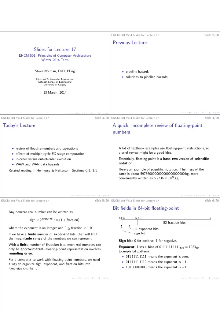
Bit fields in 64-bit floating-point Any nonzero real number can be written as sign × 2 exponent × (1 + fraction) , 63 62 52 51 0 52 fraction bits where the exponent is an integer and 0 ≤ fraction < 1 . 0. 11 exponent bits sign bit If we have a finite number of exponent bits, that will limit the magnitude range of the numbers we can represent. Sign bit: 0 for positive, 1 for negative. With a finite number of fraction bits, most real numbers can Exponent: Uses a bias of 011 1111 1111 two = 1023 ten . only be approximated —floating-point representation involves Example bit patterns: rounding error. ◮ 011 1111 1111 means the exponent is zero; For a computer to work with floating-point numbers, we need ◮ 011 1111 1110 means the exponent is − 1; a way to organize sign, exponent, and fraction bits into ◮ 100 0000 0000 means the exponent is +1. fixed-size chunks . . .

  2. slide 7/20 slide 8/20 ENCM 501 W14 Slides for Lecture 17 ENCM 501 W14 Slides for Lecture 17 63 62 52 51 0 52 fraction bits 11 exponent bits In IEEE 754 floating-point formats there are some special bit sign bit patterns: ◮ zero Fraction bits: Only bits from the right side of the “binary point” are recorded. It is assumed that there is a single 1 bit ◮ + ∞ to the left of the binary point, so that bit need not be ◮ −∞ recorded. ◮ NaN—not a number. Example: How is 1 . 375 ten represented? For example in IEEE 754, the result of 1.0/0.0 is + ∞ , but the result of 0.0/0.0 is NaN. 1 . 375 = 1 + 0 2 1 + 1 2 2 + 1 2 3 = 1 . 011 two sign, exponent, and fraction are: 0 011 1111 1111 011000 · · · 000 ENCM 501 W14 Slides for Lecture 17 slide 9/20 ENCM 501 W14 Slides for Lecture 17 slide 10/20 FP multiplication Will FP multiplication fit into a single clock cycle? If A and B are nonzero, then A × B is No! An example in textbook Section C.5 suggests a latency of signA × signB × 2 (exponentA + exponentB) 7 clock cycles for FP multiplication. × (1 + fractionA) × (1 + fractionB) The same example suggests a latency of 4 clock cycles for FP To do an FP multiplication, a logic circuit first has to check addition or subtraction, which is easier than FP multiplication, that operands are not zero or other special bit patterns. but much complicated than integer addition or subtraction. The step that costs the most time (and energy) is the Those numbers are examples . Together, Moore’s Law and 53-bit-by-53-bit integer multiplication for the ingenuity of circuit designers imply that the number vary (1 + fractionA) × (1 + fractionB). from year to year and from one design to another. At the end, there must be rounding, exponent adjustment, and a check for underflow or overflow. slide 11/20 slide 12/20 ENCM 501 W14 Slides for Lecture 17 ENCM 501 W14 Slides for Lecture 17 Fitting FP operations into the 5-stage pipeline Let’s make some notes about this picture . . . Integer unit EX Actually, this applies to fitting in integer multiplication and integer division as well. FP/integer multiply M1 M2 M3 M4 M5 M6 M7 Let’s follow the textbook example: ◮ 7-cycle latency for FP or integer multiplication IF ID MEM WB FP adder ◮ 4-cycle latency for FP addition A1 A2 A3 A4 ◮ 24-cycle latency for FP or integer division FP/integer divider (Note: Division is notoriously hard to do fast in digital logic!) DIV We are going to have to give up on our nice, easy 1-cycle EX stage in the middle of the 5-stage pipeline! Image is Figure C.35 from Hennessy J. L. and Patterson D. A., Computer Architecture: A Quantitative Approach, 5nd ed. , c � 2012, Elsevier, Inc.

  3. slide 13/20 slide 14/20 ENCM 501 W14 Slides for Lecture 17 ENCM 501 W14 Slides for Lecture 17 Quick overview of MIPS FP instructions Loads, stores and arithmetic are easy to understand. Here is a very short example: L.D F2, 0(R4) # load L.D F4, 0(R5) # load MUL.D F6, F2, F4 # multiply Many versions of the MIPS ISA have 16 64-bit floating-point S.D F6, 0(R7) # store registers: F0, F2, F4, . . . , F30—note use of even numbers only for FPRs. Note the use of GPRs for addresses. Remember, memory addresses are integers! (Newer ISA versions have 32 64-bit FPRs.) The suffix .D is for double precision . Use .S instead to work F0 is not special. Unlike the GPR R0, F0 is not hard-wired to with with 32-bit single precision FP numbers. have a value of 0.0. To understand examples in ENCM 501, we do not need to know the details of instructions for FP comparison, branching on FP comparison results, or converting between integer and FP formats. ENCM 501 W14 Slides for Lecture 17 slide 15/20 ENCM 501 W14 Slides for Lecture 17 slide 16/20 In-order versus out-of-order 5-stage pipeline with variable-length EX stage In-order execution of instructions implies that instructions are This pipeline always starts instructions in-order. This is processed in the same order that they would be in a known as in-order issue of instructions. hypothetical computer that always completes one instruction before starting the next. However, there is a design choice to be made: Should we allow instructions to complete out-of-order? The simple 5-stage pipeline is in-order , even though there are usually 5 instructions in flight within the pipeline. What are the advantages and disadvantages of forcing instruction completion to be in-order? (What about instructions that get into the 5-stage pipeline but get cancelled due to a branch?) What are some challenges created by allowing out-of-order completion? Out-of-order execution implies that start and completion of instructions is often but not always in-order . slide 17/20 slide 18/20 ENCM 501 W14 Slides for Lecture 17 ENCM 501 W14 Slides for Lecture 17 WAW (write after write) data hazards A more practical WAW hazard, and a WAR hazard WAR hazards can only occur with out-of-order issue. The WAW hazard in this example would be present only Here is a simple, but unlikely-to-occur WAW hazard: out-of-order issue. MUL.D F2, F2, F4 What are the potential hazards? L.D F2, 0(R4) MUL.D F2, F4, F6 (What is the point of the multiply if its result is going to be S.D F2, 0(R8) written over by the load?) some hazard-free instructions For program correctness the load must write to F2 after the L.D F2, 0(R9) multiply writes to F2. ADD.D F8, F8, F2 Practical WAW hazards are more likely to appear when Why are the hazards impossible in the in-order pipeline of programs do out-of-order issue . Figure C.35? What bad decision did the compiler make in generating the above code?

  4. slide 19/20 slide 20/20 ENCM 501 W14 Slides for Lecture 17 ENCM 501 W14 Slides for Lecture 17 More problems related to long latency Upcoming Topics The divide unit in the Figure C.35 has a 24-cycle latency and is not pipelined . ◮ Processing instructions with parallel pipelines. What kind of hazard is created by the lack of pipelining in the divide unit? Related reading in Hennessy & Patterson: Sections 3.1, 3.4, 3.5 What is the effect of the 4-cycle FP add latency and the 7-cycle multiply latency on the frequency and severity of RAW data hazards?

Download Presentation
Download Policy: The content available on the website is offered to you 'AS IS' for your personal information and use only. It cannot be commercialized, licensed, or distributed on other websites without prior consent from the author. To download a presentation, simply click this link. If you encounter any difficulties during the download process, it's possible that the publisher has removed the file from their server.

Recommend


More recommend