Particle Filtering Sometimes |X| is too big to use exact inference - - PowerPoint PPT Presentation

Particle Filtering

1

ØSometimes |X| is too big to use exact inference

• |X| may be too big to even store

B(X)

• E.g. X is continuous
• |X|2 may be too big to do updates

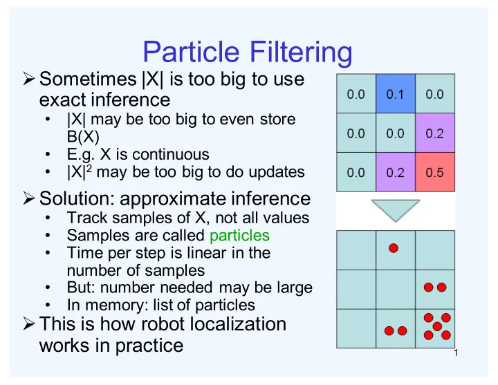
ØSolution: approximate inference

• Track samples of X, not all values
• Samples are called particles
• Time per step is linear in the

number of samples

• But: number needed may be large
• In memory: list of particles

ØThis is how robot localization works in practice

ØElapse of time

B’(Xt)=Σxt-1p(Xt|xt-1)B(xt-1) ØObserve B(Xt) ∝p(et|Xt)B’(Xt)

ØRenormalize

B(xt) sum up to 1

2

Forward algorithm vs. particle filtering

Forward algorithm Particle filtering

• Elapse of time

x--->x’

• Observe

w(x’)=p(et|x)

• Resample

resample N particles

Today

3

ØSpeech recognition

• A massive HMM!

ØIntroduction to machine learning

Speech and Language

4

ØSpeech technologies

• Automatic speech recognition (ASR)
• Text-to-speech synthesis (TTS)
• Dialog systems

ØLanguage processing technologies

• Machine translation
• Information extraction
• Web search, question answering
• Text classification, spam filtering, etc…

Digitizing Speech

5

The Input

6

ØSpeech input is an acoustic wave form

Graphs from Simon Arnfield’s web tutorial on speech, sheffield: http://www.psyc.leeds.ac.uk/research/cogn/speech/tutorial/

7

The Input

8

ØFrequency gives pitch; amplitude gives volume

• Sampling at ~8 kHz phone, ~16 kHz mic

ØFourier transform of wave displayed as a spectrogram

• Darkness indicates energy at each frequency

Acoustic Feature Sequence

9

ØTime slices are translated into acoustic feature vectors (~39 real numbers per slice) ØThese are the observations, now we need the hidden states X

State Space

10

Øp(E|X) encodes which acoustic vectors are appropriate for each phoneme (each kind of sound) Øp(X|X’) encodes how sounds can be strung together ØWe will have one state for each sound in each word ØFrom some state x, can only:

• Stay in the same state (e.g. speaking slowly)
• Move to the next position in the word
• At the end of the word, move to the start of the next word

ØWe build a little state graph for each word and chain them together to form our state space X

HMMs for Speech

11

Transitions with Bigrams

12

Decoding

13

ØWhile there are some practical issues, finding the words given the acoustics is an HMM inference problem ØWe want to know which state sequence x1:T is most likely given the evidence e1:T: ØFrom the sequence x, we can simply read off the words

( ) ( )

1: 1:

* 1: 1: 1: 1: 1:

argmax | argmax ,

T T

T T T x T T x

x p x e p x e = =

Machine Learning

14

ØUp until now: how to reason in a model and how to make optimal decisions ØMachine learning: how to acquire a model on the basis of data / experience

• Learning parameters (e.g. probabilities)
• Learning structure (e.g. BN graphs)
• Learning hidden concepts (e.g. clustering)

Parameter Estimation

15

ØEstimating the distribution of a random variable ØElicitation: ask a human ØEmpirically: use training data (learning!)

• E.g.: for each outcome x, look at the empirical rate of

that value:

• This is the estimate that maximizes the likelihood of the

data

( ) ( )

count total samples

ML

x p x =

( ) ( )

,

i i

L x p x

θ

θ =∏

( )

1 3

ML

p r =

Estimation: Smoothing

16

ØRelative frequencies are the maximum likelihood estimates (MLEs) ØIn Bayesian statistics, we think of the parameters as just another random variable, with its own distribution

( ) ( )

count total samples

ML

x p x =

( ) ( )

argmax | argmax

ML i i

p X p X

θ θ θ

θ θ = =

∏

( ) ( ) ( ) ( ) ( ) ( )

argmax | argmax | argmax |

MAP

p X p X p p X p X p

θ θ θ

θ θ θ θ θ θ = = =

????

Estimation: Laplace Smoothing

17

ØLaplace’s estimate:

• Pretend you saw every outcome
• nce more than you actually did

( ) ( )

ML LAP

p X p X = =

pLAP x

( ) =

c x

( )+1

c x

( )+1

! " # $

x

∑

= c x

( )+1

N + X

Estimation: Laplace Smoothing

18

ØLaplace’s estimate (extended):

• Pretend you saw every outcome

k extra times

• What’s Laplace with k=0?
• k is the strength of the prior

ØLaplace for conditionals:

• Smooth each condition

independently:

( ) ( ) ( )

,0 ,1 ,100 LAP LAP LAP

p X p X p X = = =

( ) ( )

,

=

LAP k

c x k p x N k X + +

( ) ( ) ( )

,

, | =

LAP k

c x y k p x y c y k X + +

Example: Spam Filter

19

Ø Input: email Ø Output: spam/ham Ø Setup:

• Get a large collection of

example emails, each labeled “spam” or “ham”

• Note: someone has to

hand label all this data!

• Want to learn to predict

labels of new, future emails

Ø Features: the attributes used to make the ham / spam decision

• Words: FREE!
• Text patterns: $dd, CAPS
• Non-text:

senderInContacts

• ……

Example: Digit Recognition

20

Ø Input: images / pixel grids Ø Output: a digit 0-9 Ø Setup:

• Get a large collection of example

images, each labeled with a digit

• Note: someone has to hand label

all this data!

• Want to learn to predict labels of

new, future digit images

Ø Features: the attributes used to make the digit decision

• Pixels: (6,8) = ON
• Shape patterns:

NumComponents, AspectRation, NumLoops

• ……

A Digit Recognizer

21

ØInput: pixel grids ØOutput: a digit 0-9

Naive Bayes for Digits

22

ØSimple version:

• One feature Fij for each grid position <i,j>
• Possible feature values are on / off, based on whether

intensity is more or less than 0.5 in underlying image

• Each input maps to a feature vector, e.g.
• Here: lots of features, each is binary valued

ØNaive Bayes model: ØWhat do we need to learn?

→ F

0,0 = 0 F 0,1 = 0 F 0,2 =1 F 0,3 =1 F 0,4 = 0 F 15,15 = 0

p Y | F

0,0F 15,15

( )∝ p Y ( )

p F

i, j |Y

( )

i, j

∏

General Naive Bayes

23

ØA general naive Bayes model: ØWe only specify how each feature depends on the class ØTotal number of parameters is linear in n

Y × F

n

parameters

p Y,F

1Fn

( ) =

p Y

( )

p F

i |Y

( )

i

∏

Y parameters n × Y × F parameters

Inference for Naive Bayes

24

ØGoal: compute posterior over causes

• Step 1: get joint probability of causes and evidence
• Step 2: get probability of evidence
• Step 3: renormalize

p Y, f1 fn

( ) =

p y1, f1 fn

( )

p y2, f1 fn

( )

 p yk, f1 fn

( )

! " # # # # # # $ % & & & & & &

p y1

( )

p fi | c1

( )

i

∏

p y2

( )

p fi | c2

( )

i

∏

 p yk

( )

p fi | ck

( )

i

∏

" # $ $ $ $ $ $ $ $ % & ' ' ' ' ' ' ' '

p f

1 f n

( )

p Y | f1 fn

( )

General Naive Bayes

25

ØWhat do we need in order to use naive Bayes?

• Inference (you know this part)
• Start with a bunch of conditionals, p(Y) and the p(Fi|Y) tables
• Use standard inference to compute p(Y|F1…Fn)
• Nothing new here
• Estimates of local conditional probability tables
• p(Y), the prior over labels
• p(Fi|Y) for each feature (evidence variable)
• These probabilities are collectively called the parameters of

the model and denoted by θ

• Up until now, we assumed these appeared by magic, but…
• … they typically come from training data: we’ll look at this now

Examples: CPTs

26

1 0.1 2 0.1 3 0.1 4 0.1 5 0.1 6 0.1 7 0.1 8 0.1 9 0.1 0.1

( )

p Y

( )

3,1

| p F

• n Y

=

1 0.05 2 0.01 3 0.90 4 0.80 5 0.90 6 0.90 7 0.25 8 0.85 9 0.60 0.80

( )

5,5

| p F

• n Y

=

1 0.01 2 0.05 3 0.05 4 0.30 5 0.80 6 0.90 7 0.05 8 0.60 9 0.50 0.80

Important Concepts

27

Ø Data: labeled instances, e.g. emails marked spam/ham

• Training set
• Held out set
• Test set

Ø Features: attribute-value pairs which characterize each x Ø Experimentation cycle

• Learn parameters (e.g. model probabilities) on training set
• (Tune hyperparameters on held-out set)
• Compute accuracy of test set
• Very important: never “peek” at the test set!

Ø Evaluation

• Accuracy: fraction of instances predicted correctly

Ø Overfitting and generalization

• Want a classifier which does well on test data
• Overfitting: fitting the training data very closely, but not

generalizing well