1 Recap: Particle Filtering Video of Demo Moderate Number of - PDF document

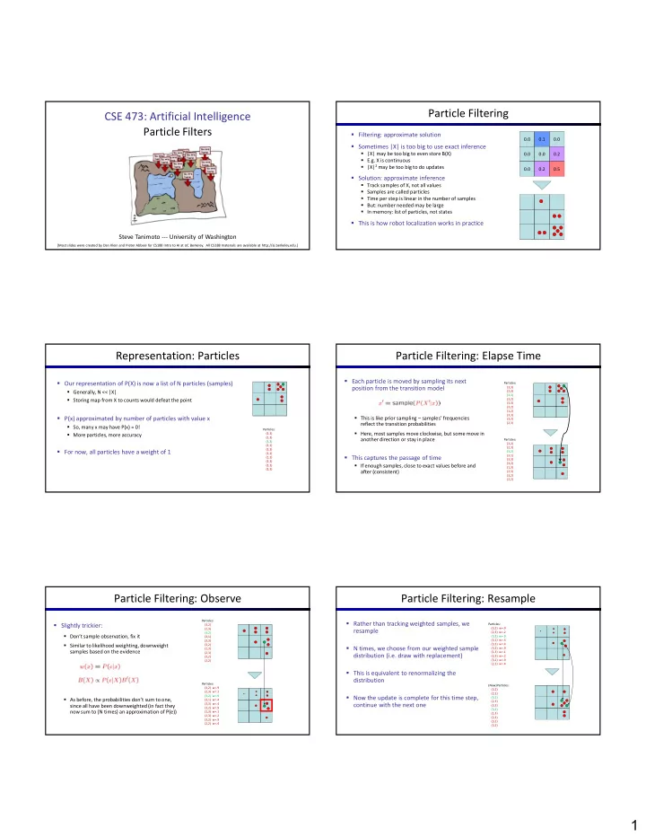
Particle Filtering CSE 473: Artificial Intelligence Particle Filters  Filtering: approximate solution 0.0 0.1 0.0  Sometimes |X| is too big to use exact inference  |X| may be too big to even store B(X) 0.0 0.0 0.2  E.g. X is continuous  |X| 2 may be too big to do updates 0.0 0.2 0.5  Solution: approximate inference  Track samples of X, not all values  Samples are called particles  Time per step is linear in the number of samples  But: number needed may be large  In memory: list of particles, not states  This is how robot localization works in practice Steve Tanimoto --- University of Washington [Most slides were created by Dan Klein and Pieter Abbeel for CS188 Intro to AI at UC Berkeley. All CS188 materials are available at http://ai.berkeley.edu.] Representation: Particles Particle Filtering: Elapse Time  Each particle is moved by sampling its next  Our representation of P(X) is now a list of N particles (samples) Particles: position from the transition model (3,3)  Generally, N << |X| (2,3) (3,3)  Storing map from X to counts would defeat the point (3,2) (3,3) (3,2) (1,2) (3,3)  P(x) approximated by number of particles with value x  This is like prior sampling – samples’ frequencies (3,3) reflect the transition probabilities (2,3)  So, many x may have P(x) = 0! Particles:  Here, most samples move clockwise, but some move in  More particles, more accuracy (3,3) (2,3) another direction or stay in place Particles: (3,3) (3,2) (3,2) (2,3) (3,3)  For now, all particles have a weight of 1 (3,2) (3,2)  This captures the passage of time (3,1) (1,2) (3,3) (3,3)  If enough samples, close to exact values before and (3,2) (3,3) (1,3) (2,3) after (consistent) (2,3) (3,2) (2,2) Particle Filtering: Observe Particle Filtering: Resample Particles:  Rather than tracking weighted samples, we  Slightly trickier: (3,2) Particles: (2,3) (3,2) w=.9 resample (2,3) w=.2 (3,2)  Don’t sample observation, fix it (3,2) w=.9 (3,1) (3,3) (3,1) w=.4  Similar to likelihood weighting, downweight (3,2) (3,3) w=.4  N times, we choose from our weighted sample (3,2) w=.9 (1,3) samples based on the evidence (1,3) w=.1 (2,3) distribution (i.e. draw with replacement) (2,3) w=.2 (3,2) (2,2) (3,2) w=.9 (2,2) w=.4  This is equivalent to renormalizing the distribution Particles: (New) Particles: (3,2) w=.9 (3,2) (2,3) w=.2 (2,2)  Now the update is complete for this time step, (3,2) w=.9 (3,2)  As before, the probabilities don’t sum to one, (3,1) w=.4 (2,3) (3,3) w=.4 continue with the next one since all have been downweighted (in fact they (3,3) (3,2) w=.9 (3,2) now sum to (N times) an approximation of P(e)) (1,3) w=.1 (1,3) (2,3) w=.2 (2,3) (3,2) w=.9 (3,2) (2,2) w=.4 (3,2) 1

Recap: Particle Filtering Video of Demo – Moderate Number of Particles  Particles: track samples of states rather than an explicit distribution Elapse Weight Resample Particles: Particles: Particles: (New) Particles: (3,3) (3,2) (3,2) w=.9 (3,2) (2,3) (2,3) (2,3) w=.2 (2,2) (3,3) (3,2) (3,2) w=.9 (3,2) (3,2) (3,1) (3,1) w=.4 (2,3) (3,3) (3,3) (3,3) w=.4 (3,3) (3,2) (3,2) (3,2) w=.9 (3,2) (1,2) (1,3) (1,3) w=.1 (1,3) (3,3) (2,3) (2,3) w=.2 (2,3) (3,3) (3,2) (3,2) w=.9 (3,2) (2,3) (2,2) (2,2) w=.4 (3,2) [Demos: ghostbusters particle filtering (L15D3,4,5)] Video of Demo – One Particle Video of Demo – Huge Number of Particles Dynamic Bayes Nets Dynamic Bayes Nets (DBNs)  We want to track multiple variables over time, using multiple sources of evidence  Idea: Repeat a fixed Bayes net structure at each time  Variables from time t can condition on those from t-1 t =1 t =2 t =3 G 1 a G 2 a G 3 a G 1 b G 2 b G 3 b E 1 a E 1 b E 2 a E 2 b E 3 a E 3 b  Dynamic Bayes nets are a generalization of HMMs [Demo: pacman sonar ghost DBN model (L15D6)] 2

DBN Particle Filters  A particle is a complete sample for a time step  Initialize : Generate prior samples for the t=1 Bayes net  Example particle: G 1a = (3,3) G 1b = (5,3)  Elapse time : Sample a successor for each particle  Example successor: G 2 a = (2,3) G 2 b = (6,3)  Observe : Weight each entire sample by the likelihood of the evidence conditioned on the sample  Likelihood: P( E 1 a | G 1 a ) * P( E 1 b | G 1 b )  Resample: Select prior samples (tuples of values) in proportion to their likelihood 3