Overview Outline: Treating Heterogeneity in PLS Path Modeling - - PowerPoint PPT Presentation

Treating Heterogeneity in PLS Path Modeling Using Latent Class Moderating Effects

Armin Monecke and Friedrich Leisch Institut f¨ ur Statistik Ludwig-Maximilians-Universit¨ at M¨ unchen

3rd Workshop on Psychometric Computing, 24.02.2011, T¨ ubingen, Germany

Overview

Outline:

• I. PLS Path Modeling
• II. Heterogeneity
• III. Moderating Effects
• IV. Latent Class Probabilities as Moderator
• V. Example: Psychosomatic Day Care Facility

PLS Path Modeling: Kick-Start

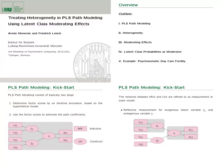
PLS Path Modeling consits of basically two steps:

• 1. Determine factor scores by an iterative procedure, based on the

hypothetical model.

• 2. Use the factor scores to estimate the path coefficients.

η ξ1 ξ2 x11 x12 y11 y12 x21 x22 MV Indicator LV Construct

PLS Path Modeling: Kick-Start

The relations between MVs and LVs are refered to as measurement or

• uter model.
• Reflective

measurement for exogenous latent variable ξ1 and endogenous variable η: η ξ1 ξ2 x11 x12 y11 y12 x21 x22

PLS Path Modeling: Kick-Start

The relations between MVs and LVs are refered to as measurement or

• uter model.
• Formative measurement for exogenous latent variable ξ2:

η ξ1 ξ2 x11 x12 y11 y12 x21 x22

PLS Path Modeling: Kick-Start

Relations between LVs are called structural or inner model. η ξ1 ξ2 x11 x12 y11 y12 x21 x22

• Exogenous variables are LVs without predecessors.
• All other LVs are endogenous.

Heterogeneity in PLS Path Models

The assumption that the data is collected from a single homogenous population is often unrealistic or may turn to be false. The presence

• f heterogeinity not accounted for may lead to biased or erroneaous

results. Within the context of PLS path modelling there are four prominent approaches to deal with heterogeneity:

• Pathmox (Sanchez & Aluja 2007): observed.
• REBUS-PLS (Esposito Vinzi et al. 2008): unobserved.
• FIMIX-PLS (Ringle et al. 2010): unobserved.
• PLS Typological Path Modeling (Squillacciotti 2010): unobserved.

Heterogeneity in PLS Path Models

All four approaches have in common to:

• 1. fit the global model,
• 2. find homogenous groups,
• 3. fit local models for each group.

Thus, the number of path coefficients increases multiplicatively with the number of groups while local sample sizes become smaller, especially, when the resulting grouping is unbalanced. Why not using the grouping indicator as a moderator variable in the global model?

Moderating Effects in PLS Path Models

Approaches for metric moderarator variables:

• Product Indicator (Chin et al. 2003)
• Two-Stage (Henseler & Fassot 2010)
• Hybrid (Wold, 1982)
• Orthogonalizing (Little et al. 2006)

Note: Moderating effects in PLS path modelling remain an open topic, especially, when nominal indicators are involved.

Product Indicator Approach

η ξ x µ ξ µ x1 x2 y1 y2 x1 · m1 x1 · m2 x2 · m1 x2 · m2 m1 m2

Two-Stage Approach

Stage 1: Run the PLS path model with only the main effects and save the estimated factor scores for further analysis. η ξ µ x1 x2 y1 y2 Stage 1 m1 m2

Two-Stage Approach

Stage 2: Calculate the interaction term ξ·µ as the element-wise product

• f the latent variable scores of the exogenous variable ξ and the

moderator variable µ. Then the path coefficients are obtained by a multiple regression on the exogenous variable η with the interaction term and the latent variable scores of ξ and µ as independent variables. η ξ · µ ξ µ ξ η Stage 2 ξ · µ µ

Other Approaches

Hybrid Approach (Wold 1982): Initially designed for estimation of models with nonlinearities in the structural model, e.g. with a quadratic term and later generalized for other nonlinearities – in particular interaction effects.

• Combination
• f

product indicator approach and two-stage approach.

• The product term ξ · µ is calculated in each iteration of the PLS-

algorithm (compare: two-stage approach).

• The product term ξ · µ is updated in each iteration (compare:

product indicator approach).

Other Approaches

Orthogonalizing Approach (Little et al. 2006): Extents the prod- uct indicator approach. But instead of the products pij, pij = xi · mj ∀ (i, j), i = 1, . . . , I, j = 1, . . . , J. the residuals ǫij (resulting from a linear regression on the main effects’ manifest variables) are used. pij = b0,ij + b1,ijx1 + · · · + bI,ijxI + bI+1,ijm1 + · · · + bI+J,ijmJ + ǫij

Latent Class Moderating Effects

To control the number of parameters we propose the following strategy:

• 1. Fit the global model and use exploratory model diagnostics to identify

set of parameters with large variability, e.g. parallel coordinate plots

• f bootstapped path coefficients.
• 2. Model

the

• verdispersion

by a convex combination

• f

several coefficient values, e.g. a finite mixture model for this subset of path coefficients. The grouping indicators are determined by a model based clustering on the respective inner models.

• 3. Refit the global model using the grouping indicators as moderator

variables for the respective path coefficients.

Example: Psychosomatic Daycare Center

. . . Structural Model F¨ ursorge Interventionen Zufriedenheit Loyalit¨ at Mitpatienten Entlassung β511 β611 β711 β111 β1112

Example: Psychosomatic Daycare Center

The facility surveyed a customer satisfaction study (N=178).

• Only

two significant (α=10%) path coefficients affecting ’Gesamtzufriedenheit’ (satisfaction) in the gloabal model: F¨ ursorge (care) → Geasmtzufriedenheit (0.51) Entlassung (release) → Geasmtzufriedenheit (0.23).

• A

priori, it was asssumed that the patients perception

• f

’Interventionen’ (psychological interventions) would be the main driver for ’Gesamtzufriedenheit’ (satisfaction).

Parallel Coordinates: Bootstrap Results

beta111 beta211 beta311 beta411 beta511 beta611 beta711 beta811 beta911 beta1011 Min Max

Components of Finite Mixture Model

Component 1: N=109 Estimate

• Std. Error

z value Pr(>|z|) (Intercept)

• 0.04

0.06

• 0.61

0.54 Fuersorge 0.49 0.08 6.21 0.00 Interventionen 0.24 0.10 2.37 0.02 Mitpatienten 0.14 0.08 1.65 0.10 Interventionen:Mitpatienten 0.04 0.04 1.01 0.31 Component 2: N=69 Estimate

• Std. Error

z value Pr(>|z|) (Intercept) 0.07 0.00 27.22 0.00 Fuersorge 0.97 0.00 324.07 0.00 Interventionen

• 0.01

0.00

• 1.99

0.05 Mitpatienten 0.00 0.00 1.07 0.29 Interventionen:Mitpatienten 0.01 0.00 4.21 0.00

Histogram: Posterior Group Probabilities

Probability for Group 1 Frequency 0.0 0.2 0.4 0.6 0.8 1.0 20 40 60 80 100

Product Terms

To construct the moderating effect we used a combination of

• the two-stage and
• the orthogonalizing approach.

p11 = GroupProbability · F¨ ursorge p12 = GroupProbability · Interventionen Resulting in the residuals of: p11 = b1 · GroupProbability + b2 · F¨ ursorge + ǫ11 p12 = b1 · GroupProbability + b2 · Interventionen + ǫ12

Path Coefficients (after & before refitting)

Path Estimate(refit) Estimate Entlassung -> Gesamtzufriedenheit 0.25 0.23 Fuersorge -> Gesamtzufriedenheit 0.60 0.51 Group -> Gesamtzufriedenheit

• 0.04

− Group*F -> Gesamtzufriedenheit

• 0.27

− Group*I -> Gesamtzufriedenheit 0.15 − Group*M -> Gesamtzufriedenheit 0.10 − Interventionen -> Gesamtzufriedenheit 0.09 0.15 Mitpatienten -> Gesamtzufriedenheit 0.08 0.11 Privatleben -> Gesamtzufriedenheit

• 0.02
• 0.07

Service -> Gesamtzufriedenheit

• 0.06
• 0.04

Parallel Coordinates: Bootstrap Results

beta115 beta515 beta615 beta715 beta815 beta915 beta1015 beta1115 beta1215 beta1315 Min Max

Summary & Open Questions

+ The proposed strategy enables the researcher to control the number

• f parameters.

+ Good interpretabilty of the moderation effects. − The selection of relevant sets of variables for the model based clustering requires a lot of expertise from the researcher.

• Can the Bootstrap Confidence Intervalls still be trusted?
• How to deal with more than two latent groups?

References

A Comparison of Approaches for the Analysis of Interaction Effects Between Latent Variables Using Partial Least Squares Path Modeling,

Henseler, J. and Chin, W. W. (2010). Structural Equation Modeling, 17:82.

Testing Moderating effects in PLS Path Models: An illustration of available procedures,

Henseler, J. and Fassot, G. (2010). In V. E. Vinzi, W. W. Chin, J. Henseler, & H. Wang (Eds.), Handbook of Partial Least Squares.

On the merits

• f
• rthogonolizing

powered and product terms: Implications for modeling interactions among latent variables,

Little, T. D., Bovaird, J.A., & Widman, K. F. (2006). Structural Equation Modeling, 13, 497-519.

Fitting Finite Mixtures of Generalized Linear Regressions in R,

Gr¨ un, B. and Leisch, F. (2007). Computational Statistics & Data Analysis 51:11, p.5247–5252.

References

semPLS: Structural Equation Modeling Using Partial Least Squares,

Monecke, A. and Leisch, F. (2010). R package version 0.8-7. 2010. http://cran. r-project.org/web/packages/semPLS/.

Histogram: Scaled PGPs

Scaled Probability for Group 1 Frequency

• 1.0
• 0.5

0.0 0.5 1.0 20 40 60 80 100