SLIDE 1 Nonlinear Signal Processing (2004/2005)
jxavier@isr.ist.utl.pt
Connectedness and compactness Definition [Connected space] Let X be a topological space. A separation
- f X is a pair of nonempty, disjoint, open subsets U, V ⊂ X such that
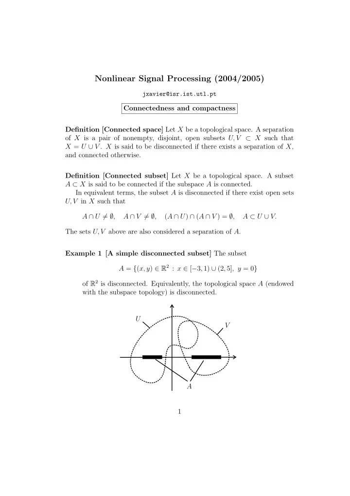
X = U ∪ V . X is said to be disconnected if there exists a separation of X, and connected otherwise. Definition [Connected subset] Let X be a topological space. A subset A ⊂ X is said to be connected if the subspace A is connected. In equivalent terms, the subset A is disconnected if there exist open sets U, V in X such that A ∩ U = ∅, A ∩ V = ∅, (A ∩ U) ∩ (A ∩ V ) = ∅, A ⊂ U ∪ V. The sets U, V above are also considered a separation of A. Example 1 [A simple disconnected subset] The subset A = {(x, y) ∈ R2 : x ∈ [−3, 1) ∪ (2, 5], y = 0}
- f R2 is disconnected. Equivalently, the topological space A (endowed
with the subspace topology) is disconnected. U V A 1
SLIDE 2 Example 2 [A more interesting disconnected subset] The subset O(n) = {X ∈ M(n, R) : XTX = In}
- f M(n, R) is disconnected. Equivalently, the topological space O(n)
(endowed with the subspace topology) is disconnected. Note that O(n) ⊂ {X ∈ M(n, R) : det X = ±1}. The open sets U = {X ∈ M(n, R) : det X < 0} V = {X ∈ M(n, R) : det X > 0} provide a separation of O(n). (Remark that O(n) ∩ U = ∅ and O(n) ∩ V = ∅; why ?) Proposition [Characterization of connectedness] A topological space X is connected if and only if the only subsets of X that are both open and closed are ∅ and X. Example 1 [Application of connectedness] Let X be a connected topo- logical space and A : X → S(n, R) a continuous map. Thus, the map x → A(x) assigns (continuously) a symmetric matrix to each point in X. Suppose the polynomial equation
n
ckA(x)k = 0 is satisfied for all x ∈ X, where ck ∈ R are fixed, real coefficients. Then, the spectrum (set of eigenvalues, including multiplicities) of A(x) is constant over x ∈ X. Proof: Pick a x0 ∈ X, let A0 = A(x0) and let σ0 = {λ1(A0), λ2(A0), . . . , λn(A0)} denote its spectrum. We assume that the eigenvalues are ordered in non-increasing order: λ1(A0) ≥ λ2(A0) ≥ · · · ≥ λn(A0). 2
SLIDE 3 Define the subset S = {x ∈ X : σ(A(x)) = σ(A0)}. Note that S = ∅ because x0 ∈ S. We will show that S is both open and closed in X. Since X is connected, this establishes that S = X by the previous proposition. To show that S is closed, let ηi : X → R, ηi(x) = λi(A(x)), for i = 1, 2, . . . , n. That is, ηi(x) computes the ith
- rdered eigenvalue of A(x). Note that each ηi is a continuous function
(composition of continuous maps). Thus, each subset Si = η−1
i (λi(A0))
is closed in X. Since S = S1∩S2∩· · ·∩Sn, it follows that S is closed in
- X. To show that S is open, we reason as follows. Let z1, z2, . . . , zm ∈ C
be the distinct roots of the polynomial equation p(z) =
n
ckzk = 0. Note that, since p(A(x)) = 0, we have λi(A(x)) ∈ {z1, z2, . . . , zm} for all i and x ∈ X. Let δ = min
k=l |zk − zl|
be the minimum distance between the distinct roots. Thus, if z ∈ {z1, z2, . . . , zm} and |z − zi| < δ, then z = zi. The subset Ui = η−1
i
((λi(Ax0) − δ, λi(Ax0) + δ)) is open in X (thanks to the continuity of ηi). By the previous argument, x ∈ Ui implies λi(A(x)) = λi(A(x0)). Thus, the open subset U = n
i=1 Ui is contained in S. But, also trivially, S ⊂ U. Thus, S = U.
Proposition [Characterization of connected subsets of R] A nonempty subset of R is connected if and only if it is an interval. Definition [Path connected space] Let X be a topological space and p, q ∈ X. A path in X from p to q is a continuous map f : [0, 1] → X such that f(0) = p and f(1) = q. 3
SLIDE 4
We say that X is path connected if for every p, q ∈ X there is a path in X from p to q. Theorem [Easy sufficient criterion for connectedness] If X is a path connected topological space, then X is connected. Example 1 [Obvious example] M(n, m, R) ≃ Rnm is connected Example 2 [Convex sets are connected] S(n, R) = {X ∈ M(n, R) : X = XT} is connected U +(n, R) = {X ∈ M(n, R) : X upper-triangular and Xii > 0} is connected Example 3 [Special orthogonal matrices] SO(n) = {X ∈ O(n) : det(X) = 1} is connected because there is a path in SO(n) from In to any X ∈ SO(n). Illustrative example: suppose X ∈ SO(5) has the eigenvalue decompo- sition X = Q cos θ − sin θ sin θ cos θ −1 −1 1 QT, Q ∈ O(n). (Note: if X ∈ SO(n) the multiplicity of the eigenvalue −1 is even.) Then, f : [0, 1] → SO(5), f(t) = Q cos(θt) − sin(θt) sin(θt) cos(θt) cos(πt) − sin(πt) sin(πt) cos(πt) 1 QT, is a path in SO(5) from I5 to X. 4
SLIDE 5 Example 4 [Non-singular matrices with positive determinant] GL+(n, R) = {X ∈ M(n, R) : det(X) > 0} is connected because there is a path in GL+(n, R) from In to any X ∈ GL+(n, R). Proof: let X ∈ GL+(n, R). Invoking the QR decomposition of X (and noting that det X > 0), we see that there exist Q ∈ SO(n) and U ∈ U+(n, R) such that X = QU. Since both SO(n) and U+(n, R) are connected, let Q(t) and U(t) be paths in SO(n) and in U+(n, R) from In to Q and U, respectively. Then, X(t) = Q(t)U(t) is a path in GL+(n, R) from In to X. Example 5 [Special Euclidean group] SE(n) = Q δ 1
- : Q ∈ SO(n), δ ∈ Rn
- is connected
because there is a path in SE(n) from In 1
Proof: let X = Q δ 1
Let Q(t) be a path in SO(n) from In to Q, and δ(t) a path in Rn from 0 to δ. Then f(t) = Q(t) δ(t) 1
Theorem [Main theorem on connectedness] Let X, Y be topological spaces and let f : X → Y be a continuous map. If X is connected, then f(X) (as a subspace of Y ) is connected. 5
SLIDE 6 Example 1 [Unit-sphere] Sn−1(R) = {x ∈ Rn : x = 1} is connected, because it is the image of the connected space Rn+1 −{0} through the continuous map f : Rn+1 − {0} → Rn f(x) = x x. Example 2 [Ellipsoid] Any non-flat ellipsoid in Rn can be described as E =
- Au + x0 : u ∈ Sn−1(R)
- where x0 ∈ Rn is the center of the ellipsoid and A ∈ GL(n, R) defines
the shape and spatial orientation of E. Thus E is connected because it is the image of the connected space Sn−1(R) through the continuous map f : Sn−1(R) → Rn f(x) = Ax + x0. Example 3 [Projective space RPn] RPn is connected because it is the image of the connected space Rn+1 − {0} through the continuous pro- jection map π : Rn+1 − {0} → RPn π(x) = [x]. Proposition [Properties of connected spaces] (a) Suppose X is a topological space and U, V are disjoint open subsets
- f X. If A is a connected subset of X contained in U ∪V , then either A ⊂ U
- r A ⊂ V .
(b) Suppose X is a topological space and A ⊂ X is connected. Then A is connected. (c) Let X be a topological space, and let {Ai} be a collection of con- nected subsets with a point in common. Then
i Ai is connected.
(d) The Cartesian product of finitely many connected topological spaces is connected. (e) Any quotient space of a connected topological space is connected. Theorem [Intermediate value theorem] Let X be a connected topolog- ical space and f is a continuous real-valued function on X. If p, q ∈ X then 6
SLIDE 7
f takes on all values between f(p) and f(q). Example 1 [Antipodal points at the same temperature] Let T : S1(R) ⊂ R2 → R be a continuous map on the unit-circle in R2. Then, there exist a point p ∈ S1(R) such that T(p) = T(−p). Proof: The map f : [0, 2π] → R f(θ) = T(cos θ, sin θ) − T(− cos θ, − sin θ) is continuous. If f(0) = 0, we can pick p = (1, 0). Otherwise, f(0)f(π) < 0 and there exists θ0 ∈ [0, π] such that f(θ0) = 0. Make p = (cos θ0, sin θ0). As a consequence, this shows that there two antipodal points in the Earth’s equator line at the same temperature. Definition [Components] Let X be a topological space. A component of X is a maximally connected subset of X, that is, a connected set that is not contained in any larger connected set. ⊲ Intuition: X consists of a union of disjoint “islands”/components. Example 1 [Orthogonal group] The orthogonal group O(n) = {X ∈ M(n, R) : XTX = In} has two components: SO(n) = {X ∈ O(n, R) : det X = 1} O−(n) = {X ∈ O(n, R) : det X = −1}. Proof: We have already seen that SO(n) is connected. Any attempt to enlarge SO(n) involves taking a point in O−(n). But, then, the sets U = {X ∈ M(n, R) : det X < 0} and V = {X ∈ M(n, R) : det X > 0} 7
SLIDE 8 would provide a separation of such set. Thus, SO(n) is a component
- f O(n). The set O−(n) is connected because it is the image of SO(n)
through the continuous map f : SO(n) → M(n, R) f(X) = −1 1 ... 1 X. Thus, O−(n) is a component of O(n). Proposition [Properties of components] Let X be any topological space. (a) Each component of X is closed in X. (b) Any connected subset of X is contained in a single component. Definition [Compact space] A topological space X is said to be compact if every open cover of X has a finite subcover. That is, if U is any given
- pen cover of X, then there are finitely many sets U1, . . . , Uk ∈ U such that
X = U1 ∪ · · · ∪ Uk. Definition [Compact subset] Let X be a topological space. A subset A ⊂ X is said to be compact if the subspace A is compact. In equivalent terms, the subset A is compact if and only if given any collection of open subsets of X covering A, there is a finite subcover. Proposition [Characterization of compact sets in Rn] A subset X in Rn is compact if and only if X is closed and bounded. Example 1 [Stiefel manifold] The set O(n, m) = {X ∈ M(n, m, R) : XTX = Im} is compact because it is closed and bounded. 8
SLIDE 9 It is closed because O(n, m) = f −1({Im}) and f : M(n, m, R) → M(m, R) f(X) = XTX is continuous. It is bounded because, if X ∈ O(n, m) then X2 = tr(XTX) = tr(Im) = m. Note that O(n, 1) = Sn−1(R) and O(n, n) = O(n). Theorem [Main theorem on compactness] Let X, Y be topological spaces and let f : X → Y be a continuous map. If X is compact, then f(X) (as a subspace of Y ) is compact. Example 1 [Projective space RPn] The projective space RPn is compact because it is the image of the compact set Sn(R) through the continuous projection map π : Rn+1 − {0} → RPn. Proposition [Properties of compact spaces] (a) Every closed subset of a compact space is compact. (b) In a Hausdorff space X, compact sets can be separated by open
- sets. That is, if A, B ⊂ X are disjoint compact subsets, there exist disjoint
- pen sets U, V ⊂ X such that A ⊂ U and B ⊂ V .
(c) Every compact subset of a Hausdorff space is closed. (d) The Cartesian product of finitely many compact topological spaces is compact. (e) Any quotient space of a compact topological space is compact. Example 1 [Special orthogonal matrices] SO(n) = {X ∈ O(n) : det X = 1} 9
SLIDE 10 is compact because it is a closed subset of the compact space O(n). It is closed because SO(n) = f −1({1}) and f : O(n) → R f(X) = det X is continuous. Theorem [Extreme value theorem] If X is a compact space and f : X → R is continuous, then f attains its maximum and minimum values
Proposition [Characterization of compactness in 2nd countable Haus- dorff spaces] Let X be a 2nd countable Hausdorff space. The following are equivalent: (a) X is compact (b) Every sequence of points in X has a subsequence that converges to a point in X. Example 1 [Principal component analysis is a continuous map] Let X, Y be 2nd countable Hausdorff spaces. Furthermore, let Y be com-
- pact. Let F : X × Y → R be a continuous function. For each x ∈ X,
we define the function Fx : Y → R, Fx(y) = F(x, y). Suppose that, for each x ∈ X, there exists only one global minimizer in Y of the function Fx. Let φ : X → Y be the map which, given x ∈ X, returns the (unique) global minimizer in Y of the function Fx. The map φ is continuous. Proof: In this topological setting, it suffices to prove that xn → x0 implies yn = φ(xn) → y0 = φ(x0). Suppose yn → y0 (we will reach a contradiction). Then, there exists an open set U in Y containing y0 and a subsequence ynk such that ynk ∈ U. Since Y is compact, the sequence ynk admits a convergent subsequence, say, ynkl → z. Now, we claim z = y0. To show this, choose y ∈ Y arbitrarily. We have F(xnkl, ynkl) ≤ F(xnkl, y) for all l. 10
SLIDE 11 Taking the limit l → ∞ yields F(x0, z) ≤ F(x0, y). Since y was chosen arbitrarily, this shows that z is a global minimizer
- f Fx0. By uniqueness, z = y0. Since the sequence ynkl → z = y0 it has
a point in U (contradiction!). Let P = [ p1 p2 . . . pk] ∈ M(n, k, R) denote a constellation of k points in Rn. A one-dimensional principal component analysis (PCA) of P consists in extracting the “dominant” straight line in P. That is, the straight line spanned by a vector
∈ arg min x ∈ Rn − {0}
k
x2pj
= arg max x ∈ Rn − {0} xTPP Tx x2 . The straight line is unique if λmax(PP T) is simple. In equivalent terms,
- rder the eigenvalues of the n × n symmetric matrix PP T as
λn(PP T)
≤ λn−1(PP T) ≤ · · · ≤ λ2(PP T) ≤ λ1(PP T)
. The dominant straight line is unique for those constellations P belong- ing to P =
- P ∈ M(n, k, R) : λ1(PP T) > λ2(PP T)
- .
Since each λj : S(n, R) → R is a continuous function on S(n, R), the set of n × n symmetric matrices with real entries (see your homework for this result!), the set P is open in M(n, k, R). Thus, we have a map PCA : P → RPn−1 P ∈ P PCA π( x(P)) ∈ RPn−1 The map PCA is continuous, because 11
SLIDE 12 Step 1: The map F : RPn−1 × M(n, k, R) → R F([x], P) =
k
x2pj
is continuous (as we have already seen in a previous example). Step 2: Its restriction to the subspace RPn−1×P ⊂ RPn−1×M(n, k, R) is also continuous (for brevity of notation, we keep the same symbol F): F : RPn−1 × P → R F([x], P) =
k
x2pj
. Step 3: PCA : P → RPn−1 extracts, for each P ∈ P, the (unique) minimizer of FP in RPn−1. Since RPn−1 is compact, the previous result shows that PCA is continuous.
References
[1] J. Lee, Introduction to Topological Manifolds, Springer-Verlag, 2000. 12