Lecture 5: Basic Dynamical Systems CS 344R/393R: Robotics - - PDF document

1

Lecture 5: Basic Dynamical Systems

CS 344R/393R: Robotics Benjamin Kuipers

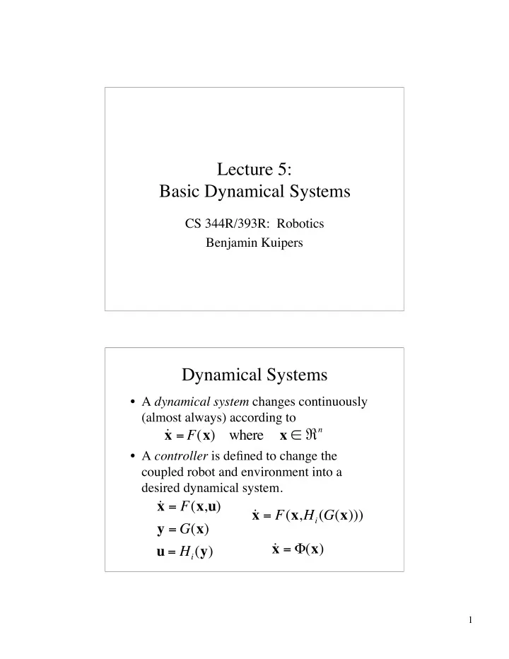
Dynamical Systems

• A dynamical system changes continuously

(almost always) according to

• A controller is defined to change the

coupled robot and environment into a desired dynamical system.

˙ x = F(x) where x

n

˙ x = F(x,u) y = G(x) u = Hi(y) ˙ x = F(x,Hi(G(x))) ˙ x = (x)

2

Two views of dynamic behavior

• Time

plot (t,x)

• Phase

portrait (x,v)

Phase Portrait: (x,v) space

• Shows the trajectory (x(t),v(t)) of the system

– Stable attractor here

3

Interesting Phase Portrait

• The van der Pol equation has a limit cycle.

˙ ˙ x µ(1 x 2) ˙ x + x = 0

In One Dimension

• Simple linear system
• Fixed point
• Solution

– Stable if k < 0 – Unstable if k > 0

˙ x = kx

x = 0

• ˙

x = 0

x ˙ x

x(t) = x0 e

kt

4

In Two Dimensions

• Often, we have position and velocity:
• If we model actions as forces, which cause

acceleration, then we get: x = (x,v)

T

where v = ˙ x

˙ x = ˙ x ˙ v

• =

˙ x ˙ ˙ x

• =

v forces

• The Damped Spring
• The spring is defined by Hooke’s Law:
• Include damping friction
• Rearrange and redefine constants

x k x m ma F

1

• =

= = & &

x k x k x m & & &

2 1

• =

= + + cx x b x & & & ˙ x = ˙ x ˙ v

• =

˙ x ˙ ˙ x

• =

v b˙ x cx

5

The Linear Spring Model

• Solutions are:
• Where r1, r2 are roots of the characteristic

equation

˙ ˙ x + b˙ x + cx = 0

• 2 + b + c = 0

r

1,r2 = b ±

b2 4c 2

x(t) = Ae

r

1t + Be

r2t

c 0

Qualitative Behaviors

• Re(r1), Re(r2) < 0

means stable.

• Re(r1), Re(r2) > 0

means unstable.

• b2-4c < 0 means

complex roots, means oscillations.

b c unstable stable spiral nodal nodal unstable

r

1,r2 = b ±

b2 4c 2

6

It’s the same in higher dimensions

• The characteristic equation for

generalizes to

– This means that there is a vector v such that

• The solutions are called eigenvalues.
• The related vectors v are eigenvectors.

˙ x = Ax

det( A I) = 0

Av = v

• Qualitative Behavior, Again
• For a dynamical system to be stable:

– The real parts of all eigenvalues must be negative. – All eigenvalues lie in the left half complex plane.

• Terminology:

– Underdamped = spiral (some complex eigenvalue) – Overdamped = nodal (all eigenvalues real) – Critically damped = the boundary between.

7

Node Behavior Focus Behavior

8

Saddle Behavior Spiral Behavior (stable attractor)

9

Center Behavior (undamped

• scillator)

The Wall Follower

(x,y)

10

The Wall Follower

• Our robot model:

u = (v ω)T y=(y θ)T θ ≈ 0.

• We set the control law u = (v ω)T = Hi(y)

˙ x = ˙ x ˙ y ˙

• = F(x,u) =

vcos vsin

• e = y yset

so ˙ e = ˙ y and ˙ ˙ e = ˙ ˙ y

The Wall Follower

• Assume constant forward velocity v = v0

– approximately parallel to the wall: θ ≈ 0.

• Desired distance from wall defines error:
• We set the control law u = (v ω)T = Hi(y)

– We want e to act like a “damped spring”

e = y yset so ˙ e = ˙ y and ˙ ˙ e = ˙ ˙ y

˙ ˙ e + k1 ˙ e + k2 e = 0

11

The Wall Follower

• We want
• For small values of θ
• Assume v=v0 is constant. Solve for ω

– This makes the wall-follower a PD controller.

˙ ˙ e + k1 ˙ e + k2 e = 0

˙ e = ˙ y = vsin

• v

˙ ˙ e = ˙ ˙ y = vcos ˙

• v

u = v

• =

v0 k1 k2 v0 e

• = Hi(e,)

Tuning the Wall Follower

• The system is
• Critical damping requires
• Slightly underdamped performs better.

– Set k2 by experience. – Set k1 a bit less than

˙ ˙ e + k1 ˙ e + k2 e = 0

k

1 2 4k2 = 0

k

1 =

4k2

4k2

12

An Observer for Distance to Wall

• Short sonar returns are reliable.

– They are likely to be perpendicular reflections.

Experiment with Alternatives

• The wall follower is a PD control law.
• A target seeker should probably be a PI

control law, to adapt to motion.

• Try different tuning values for parameters.

– This is a simple model. – Unmodeled effects might be significant.

13

Ziegler-Nichols Tuning

• Open-loop response to a unit step increase.
• d is deadtime. T is the process time constant.
• K is the process gain.

d T K

Tuning the PID Controller

• We have described it as:
• Another standard form is:
• Ziegler-Nichols says:

u(t) = kP e(t) kI edt

t

• kD ˙

e (t) u(t) = P e(t) + TI edt

t

• + TD˙

e (t)

• P = 1.5 T

K d TI = 2.5 d TD = 0.4 d

14

Ziegler-Nichols Closed Loop

• 1. Disable D and I action (pure P control).
• 2. Make a step change to the setpoint.
• 3. Repeat, adjusting controller gain until

achieving a stable oscillation.

• This gain is the “ultimate gain” Ku.
• The period is the “ultimate period” Pu.

Closed-Loop Z-N PID Tuning

• A standard form of PID is:
• For a PI controller:
• For a PID controller:

u(t) = P e(t) + TI edt

t

• + TD˙

e (t)

• P = 0.45 Ku

TI = P

u

1.2 P = 0.6 Ku TI = P

u

2 TD = P

u

8

15

Summary of Concepts

• Dynamical systems and phase portraits
• Qualitative types of behavior

– Stable vs unstable; nodal vs saddle vs spiral – Boundary values of parameters

• Designing the wall-following control law
• Tuning the PI, PD, or PID controller

– Ziegler-Nichols tuning rules – For more, Google: controller tuning