ANALYSIS of EUCLIDEAN ALGORITHMS An Arithmetical Instance of - - PowerPoint PPT Presentation

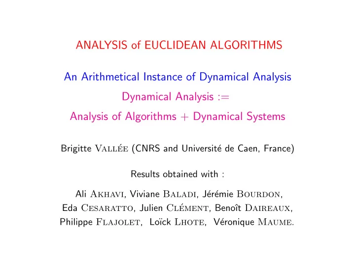
ANALYSIS of EUCLIDEAN ALGORITHMS An Arithmetical Instance of Dynamical Analysis Dynamical Analysis := Analysis of Algorithms + Dynamical Systems

Brigitte Vall´ ee (CNRS and Universit´ e de Caen, France) Results obtained with : Ali Akhavi, Viviane Baladi, J´ er´ emie Bourdon, Eda Cesaratto, Julien Cl´ ement, Benoˆ ıt Daireaux, Philippe Flajolet, Lo¨ ıck Lhote, V´ eronique Maume.

Plan of the Talk I– The Euclid Algorithm, and the underlying dynamical system II– The other Euclidean Algorithms III– Probabilistic –and dynamical– analysis of algorithms IV– Euclidean algorithms : the underlying dynamical systems V– Dynamical analysis of Euclidean algorithms

Plan of the Talk I– The Euclid Algorithm, and the underlying dynamical system II– The other Euclidean Algorithms III– Probabilistic –and dynamical– analysis of algorithms IV– Euclidean algorithms : the underlying dynamical systems V– Dynamical analysis of Euclidean algorithms

The (standard) Euclid Algorithm: the grand father of all the algorithms. On the input (u, v), it computes the gcd of u and v, together with the Continued Fraction Expansion of u/v.

The (standard) Euclid Algorithm: the grand father of all the algorithms. On the input (u, v), it computes the gcd of u and v, together with the Continued Fraction Expansion of u/v. u0 := v; u1 := u; u0 ≥ u1                u0 = m1u1 + u2 0 < u2 < u1 u1 = m2u2 + u3 0 < u3 < u2 . . . = . . . + up−2 = mp−1up−1 + up 0 < up < up−1 up−1 = mpup + up+1 = 0                up is the gcd of u and v, the mi’s are the digits. p is the depth.

The (standard) Euclid Algorithm: the grand father of all the algorithms. On the input (u, v), it computes the gcd of u and v, together with the Continued Fraction Expansion of u/v. u0 := v; u1 := u; u0 ≥ u1                u0 = m1u1 + u2 0 < u2 < u1 u1 = m2u2 + u3 0 < u3 < u2 . . . = . . . + up−2 = mp−1up−1 + up 0 < up < up−1 up−1 = mpup + up+1 = 0                up is the gcd of u and v, the mi’s are the digits. p is the depth. CFE of u v : u v = 1 m1 + 1 m2 + 1 ... + 1 mp ,

The underlying Euclidean dynamical system (I). The trace of the execution of the Euclid Algorithm on (u1, u0) is: (u1, u0) → (u2, u1) → (u3, u2) → . . . → (up−1, up) → (up+1, up) = (0, up)

The underlying Euclidean dynamical system (I). The trace of the execution of the Euclid Algorithm on (u1, u0) is: (u1, u0) → (u2, u1) → (u3, u2) → . . . → (up−1, up) → (up+1, up) = (0, up) Replace the integer pair (ui, ui−1) by the rational xi := ui ui−1 . The division ui−1 = miui + ui+1 is then written as xi+1 = 1 xi − 1 xi

• r

xi+1 = T(xi), where T : [0, 1] − → [0, 1], T(x) := 1 x − 1 x

• for x = 0,

T(0) = 0

The underlying Euclidean dynamical system (I). The trace of the execution of the Euclid Algorithm on (u1, u0) is: (u1, u0) → (u2, u1) → (u3, u2) → . . . → (up−1, up) → (up+1, up) = (0, up) Replace the integer pair (ui, ui−1) by the rational xi := ui ui−1 . The division ui−1 = miui + ui+1 is then written as xi+1 = 1 xi − 1 xi

• r

xi+1 = T(xi), where T : [0, 1] − → [0, 1], T(x) := 1 x − 1 x

• for x = 0,

T(0) = 0 An execution of the Euclidean Algorithm (x, T(x), T 2(x), . . . , 0) = A rational trajectory of the Dynamical System ([0, 1], T) = a trajectory that reaches 0. The dynamical system is a continuous extension of the algorithm.

T(x) := 1 x − 1 x

• T[m] :]

1 m + 1, 1 m[− →]0, 1[, T[m](x) := 1 x − m h[m] :]0, 1[− →] 1 m + 1, 1 m[ h[m](x) := 1 m + x

The Euclidean dynamical system (II). A dynamical system with a denumerable system of branches (T[m])m≥1, T[m] :] 1 m + 1, 1 m[− →]0, 1[, T[m](x) := 1 x − m The set H of the inverse branches of T is H := { h[m] :]0, 1[− →] 1 m + 1, 1 m[; h[m](x) := 1 m + x}

The Euclidean dynamical system (II). A dynamical system with a denumerable system of branches (T[m])m≥1, T[m] :] 1 m + 1, 1 m[− →]0, 1[, T[m](x) := 1 x − m The set H of the inverse branches of T is H := { h[m] :]0, 1[− →] 1 m + 1, 1 m[; h[m](x) := 1 m + x} The set H builds one step of the CF’s. The set Hn of the inverse branches of T n builds CF’s of depth n. The set H⋆ := Hn builds all the (finite) CF’s.

u v = 1 m1 + 1 m2 + 1 ... + 1 mp = h[m1] ◦ h[m2] ◦ . . . ◦ h[mp](0)

The Euclidean dynamical system (III). Density Transformer: For a density f on [0, 1], H[f] is the density on [0, 1] after one iteration of the shift H[f](x) =

• h∈H

|h′(x)| f◦h(x) =

• m∈N

1 (m + x)2 f( 1 m + x).

The Euclidean dynamical system (III). Density Transformer: For a density f on [0, 1], H[f] is the density on [0, 1] after one iteration of the shift H[f](x) =

• h∈H

|h′(x)| f◦h(x) =

• m∈N

1 (m + x)2 f( 1 m + x). Transfer operator (Ruelle): Hs[f](x) =

• h∈H

|h′(x)|s f ◦ h(x).

The Euclidean dynamical system (III). Density Transformer: For a density f on [0, 1], H[f] is the density on [0, 1] after one iteration of the shift H[f](x) =

• h∈H

|h′(x)| f◦h(x) =

• m∈N

1 (m + x)2 f( 1 m + x). Transfer operator (Ruelle): Hs[f](x) =

• h∈H

|h′(x)|s f ◦ h(x). The k-th iterate satisfies: Hk

s[f](x) =

• h∈Hk

|h′(x)|s f ◦ h(x)

Plan of the Talk I– The Euclid Algorithm, and the underlying dynamical system II– The other Euclidean Algorithms III– Probabilistic –and dynamical– analysis of algorithms IV– Euclidean algorithms : the underlying dynamical systems V– Dynamical analysis of Euclidean algorithms

Many variants of the Euclid Algorithm.

A Euclidean algorithm:= any algorithm which performs a sequence of divisions v = mu + r. There are various possible types of Euclidean divisions – MSB divisions [directed by the Most Significant Bits] shorten integers on the left, and provide a remainder r smaller than u, (w.r.t the usual absolute value), i.e. with more zeroes on the left. – LSB divisions [directed by the Least Significant Bits] shorten integers on the right, and provide a remainder r smaller than u (w.r.t the dyadic absolute value), i.e. with more zeroes on the right. – Mixed divisions shorten integers both on the right and on the left, with new zeroes both on the right and on the left.

Instances of MSB Algorithms.

– Variants according to the position of remainder r, By Default: v = mu + r with 0 ≤ r < u By Excess: v = mu − r with 0 ≤ r < u Centered: v = mu + ǫr with ǫ = ±1, 0 ≤ r ≤ u/2

Instances of MSB Algorithms.

– Variants according to the position of remainder r, By Default: v = mu + r with 0 ≤ r < u By Excess: v = mu − r with 0 ≤ r < u Centered: v = mu + ǫr with ǫ = ±1, 0 ≤ r ≤ u/2 – Subtractive Algorithm : A division with quotient m can be replaced by m subtractions While v ≥ u do v := v − u

An instance of a Mixed Algorithm.

The Subtractive Algorithm, where the zeroes on the right are removed from the remainder defines the Binary Algorithm. Subtractive Gcd Algorithm. Binary Gcd Algorithm.

• Input. u, v; v ≥ u
• Input. u, v odd; v ≥ u

While (u = v) do While (u = v) do While v > u do While v > u do k := ν2(v − u); v := v − u v := v − u 2k ; Exchange u and v. Exchange u and v.

• Output. u (or v).
• Output. u (or v).

The 2-adic valuation ν2 counts the number of zeroes on the right

An instance of a LSB Algorithm.

On a pair (u, v) with v odd and u even, with ν2(u) = k, of the form u := 2k u′ the LSB division writes v = a · u′ + 2k · r′, with ν2(r′) > ν2(u′) = 0 and gcd(u, v) = gcd(r′, u′). The pair (u′, r′) will be the new pair for the next step.

An execution of the LSB Algorithm:

the Tortoise and the Hare

10001100101000001 1 111101011000000101000 2 11001001101101010000 3 110000110001010000000 4 10011000111100000000 5 111010010101000000000 6 110000010010000000000 7 100010001100000000000 8 1000001011000000000000 9 1100000000000000 10 1000001000000000000000 11 100010000000000000000 12 110000000000000000000 13 10000000000000000000000

Three main outputs for any Euclidean Algorithm

– the gcd(u, v) itself Essential in exact rational computations, for keeping rational numbers under their irreducible forms 60% of the computation time in some symbolic computations

Three main outputs for any Euclidean Algorithm

– the gcd(u, v) itself Essential in exact rational computations, for keeping rational numbers under their irreducible forms 60% of the computation time in some symbolic computations – the Continued Fraction Expansion CFE (u/v) Often used directly in computation over rationals.

Three main outputs for any Euclidean Algorithm

– the gcd(u, v) itself Essential in exact rational computations, for keeping rational numbers under their irreducible forms 60% of the computation time in some symbolic computations – the Continued Fraction Expansion CFE (u/v) Often used directly in computation over rationals. – the modular inverse u−1 mod v, when gcd(u, v) = 1. Extensively used in cryptography

A basic algorithm ... Perhaps the fifth main operation?

Main algorithmic questions.

– Analyse the behaviour of these various Euclidean algorithms – Compare them with respect to various costs and particularly the bit–complexity. Experimental comparison

• f bit–complexities.

A gaussian law for the number of steps?

Comparison for five algorithms on the input (2011176, 72001) Evolution of the remainders

Standard Centered By-Excess Binary LSB 67149 4852 4852 44849 51637 4852 779 779 1697 12485 4073 178 601 1697 2447 779 67 423 125 3733 178 23 245 125 1545 67 2 67 9 547 44 1 23 9 523 23 – 2 5 3 19 – 1 1 65 4 – – – 17 3 – – – 3 1 – – – 1

Comparison for five algorithms on the input (2011176, 72001) Evolution of the remainders

Standard Centered By-Excess Binary LSB 67149 4852 4852 44849 51637 4852 779 779 1697 12485 4073 178 601 1697 2447 779 67 423 125 3733 178 23 245 125 1545 67 2 67 9 547 44 1 23 9 523 23 – 2 5 3 19 – 1 1 65 4 – – – 17 3 – – – 3 1 – – – 1

Explain the behaviour of algorithms

For instance, an execution of the LSB Algorithm : the Tortoise and the Hare 10001100101000001 1 111101011000000101000 2 11001001101101010000 3 110000110001010000000 4 10011000111100000000 5 111010010101000000000 6 110000010010000000000 7 100010001100000000000 8 1000001011000000000000 9 1100000000000000 10 1000001000000000000000 11 100010000000000000000 12 110000000000000000000 13 10000000000000000000000

Plan of the Talk I– The Euclid Algorithm, and the underlying dynamical system II– The other Euclidean Algorithms III– Probabilistic –and dynamical– analysis of algorithms IV– Euclidean algorithms : the underlying dynamical systems V– Dynamical analysis of Euclidean algorithms

Probabilistic Analysis of Algorithms

An algorithm with a set of inputs Ω, and a parameter (or a cost) C defined on Ω which describes – the execution of the algorithm (number of iterations, bit–complexity) – or the geometry of the output (here: the continued fraction)

Probabilistic Analysis of Algorithms

An algorithm with a set of inputs Ω, and a parameter (or a cost) C defined on Ω which describes – the execution of the algorithm (number of iterations, bit–complexity) – or the geometry of the output (here: the continued fraction) – Gather the inputs wrt to their sizes (here, their number of bits) Ωn := {(u, v) ∈ Ω, size(u, v) = n}. – Consider a distribution on Ωn (for instance the uniform distribution), – Study the cost C on Ωn in a probabilistic way: – Estimate the mean value of Cn := C|Ωn, its variance, its distribution... in an asymptotic way (for n → ∞)

The main costs of interest for Euclidean Algorithms

– The additive costs, which depend on the digits C(u, v) :=

p

• i=1

c(mi) if c = 1, then C := the number of iterations if c = 1m0, then C := the number of digits equal to m0 if c = ℓ (the binary length), then C := the length of the CFE

The main costs of interest for Euclidean Algorithms

– The additive costs, which depend on the digits C(u, v) :=

p

• i=1

c(mi) if c = 1, then C := the number of iterations if c = 1m0, then C := the number of digits equal to m0 if c = ℓ (the binary length), then C := the length of the CFE – The bit complexity (not an additive cost) C(u, v) :=

p

• i=1

ℓ(ui) ℓ(mi)

The results (I) Previous results

– mostly in the average-case, – only for the number of iterations, and specific to particular algorithms... – well–described in Knuth’s book (Tome II)

The results (I) Previous results

– mostly in the average-case, – only for the number of iterations, and specific to particular algorithms... – well–described in Knuth’s book (Tome II) Heilbronn, Dixon, Rieger (70): Standard and Centered Alg. Yao and Knuth (75): Subtractive Alg. Brent (78): Binary Alg (partly heuristic), Hensley (94) : A distributional study for the Standard Alg. Stehl´ e and Zimmermann (05) : LSB Alg (experiments)

The new results

With Dynamical Analysis method, our group [1995 → now ] obtains

The new results

With Dynamical Analysis method, our group [1995 → now ] obtains – a complete classification into two classes, – the Fast Class ={Standard, Centered, Binary, LSB}, – the Slow Class = {By-Excess, Subtractive}.

The new results

With Dynamical Analysis method, our group [1995 → now ] obtains – a complete classification into two classes, – the Fast Class ={Standard, Centered, Binary, LSB}, – the Slow Class = {By-Excess, Subtractive}. – an average-case analysis of a broad class of costs, – all the additive costs – and also the bit–complexity.

The new results

With Dynamical Analysis method, our group [1995 → now ] obtains – a complete classification into two classes, – the Fast Class ={Standard, Centered, Binary, LSB}, – the Slow Class = {By-Excess, Subtractive}. – an average-case analysis of a broad class of costs, – all the additive costs – and also the bit–complexity. – a distributional analysis of a subclass of the Fast Class, the Good Class = {Standard, Centered}. Asymptotic gaussian laws hold for: – P, and additive costs of moderate growth, – the remainder size log ui for i ∼ δP, – the bit-complexity of the extended Alg.

Here, focus on average-case results (n := input size)

Here, focus on average-case results (n := input size) – For the Fast Class ={Standard, Centered, Binary, LSB } , – the mean values of costs P, C are linear wrt n, – the mean bit-complexity is quadratic. En[P] ∼ 2 log 2 h(S) n, En[C] ∼ 2 log 2 h(S) µ[c] n, En[B] ∼ log 2 h(S)µ[ℓ] n2.

h(S) is the entropy of the system, µ[c] the mean value of step–cost c.

– Moreover, these costs are concentrated: En[Ck] ∼ En[C]k

Here, focus on average-case results (n := input size) – For the Fast Class ={Standard, Centered, Binary, LSB } , – the mean values of costs P, C are linear wrt n, – the mean bit-complexity is quadratic. En[P] ∼ 2 log 2 h(S) n, En[C] ∼ 2 log 2 h(S) µ[c] n, En[B] ∼ log 2 h(S)µ[ℓ] n2.

h(S) is the entropy of the system, µ[c] the mean value of step–cost c.

– Moreover, these costs are concentrated: En[Ck] ∼ En[C]k – For the Slow Class = {By-Excess, Subtractive}, – the mean values of costs P, C are quadratic, – the mean bit-complexity of B is cubic, – the moments of order k ≥ 2 are exponential: En[Ck] = Θ(2n(k−1)).

The main constant h(S) is the entropy of the Dynamical System. A well-defined mathematical object, computable.

The main constant h(S) is the entropy of the Dynamical System. A well-defined mathematical object, computable. – Related to classical constants for the first two algs h(S) = π2 6 log 2 ∼ 2.37 [Standard], h(S) = π2 6 log φ ∼ 3.41 [Centered].

The main constant h(S) is the entropy of the Dynamical System. A well-defined mathematical object, computable. – Related to classical constants for the first two algs h(S) = π2 6 log 2 ∼ 2.37 [Standard], h(S) = π2 6 log φ ∼ 3.41 [Centered]. – For the LSB alg, h(S) = 4−2γ ∼ 3.91 involves the Lyapounov exponent γ of the set of random matrices, where Na,k = 1 2k

• 2k

2k a

• with k ≥ 1, a odd, |a| < 2k is taken with prob. 2−2k,

The main constant h(S) is the entropy of the Dynamical System. A well-defined mathematical object, computable. – Related to classical constants for the first two algs h(S) = π2 6 log 2 ∼ 2.37 [Standard], h(S) = π2 6 log φ ∼ 3.41 [Centered]. – For the LSB alg, h(S) = 4−2γ ∼ 3.91 involves the Lyapounov exponent γ of the set of random matrices, where Na,k = 1 2k

• 2k

2k a

• with k ≥ 1, a odd, |a| < 2k is taken with prob. 2−2k,

– For the Binary alg, h(S) = π2f(1) ∼ 3.6 involves the value f(1) of the unique density which satisfies the functional equation f(x) =

• k≥1
• a odd

1≤a<2k

• 1

2kx + a 2 f

• 1

2kx + a

Precise comparisons between the four Fast Algorithms Algs Nb of iterations Bit-complexity Standard 0.584 n 1.242 n2 Centered 0.406 n 1.126 n2 (Ind.) Binary 0.381 n 0.720 n2 LSB 0.511 n 1.115 n2

Main principles of Dynamical Analysis := Analysis of Algorithms + Dynamical Systems

1– Interaction between the discrete world and the continuous world. Three steps. (a) The discrete algorithm is extended into a continuous process..... (b) .... which is studied – more easily, using all the analytic tools.

1– Interaction between the discrete world and the continuous world. Three steps. (a) The discrete algorithm is extended into a continuous process..... (b) .... which is studied – more easily, using all the analytic tools. (c) Returning to the discrete algorithm, with various principles of transfer from continuous to discrete. The discrete data are of zero measure amongst the continuous data.

Main tools for probabilistic analysis of algorithms 2– Generating functions ? A classical tool : Generating functions of various types A(z) :=

• n≥0

anzn, ˆ A(z) :=

• n≥0

an zn n! ,

• A(s) :=
• n≥1

an ns Directly used when the distribution of data does not change too much during the execution of the algorithm (for instance: the Euclid Algorithm on polynomials)

Main tools for probabilistic analysis of algorithms 2– Generating functions ? A classical tool : Generating functions of various types A(z) :=

• n≥0

anzn, ˆ A(z) :=

• n≥0

an zn n! ,

• A(s) :=
• n≥1

an ns Directly used when the distribution of data does not change too much during the execution of the algorithm (for instance: the Euclid Algorithm on polynomials) Here, this is not the case .... due to the existence of the carries The study of the dynamical system underlying the algorithm explains how the distribution of data evolves during the execution of the algorithm. It also describes the behaviour of the generating functions of costs...

Main tools for probabilistic analysis of algorithms 3- Dynamical Analysis –main principles. Input.- A discrete algorithm. Step 1.- Extend the discrete algorithm into a continuous process, i.e. a dynamical system. (X, V ) X compact, V : X → X, where the discrete alg. gives rise to particular trajectories.

Main tools for probabilistic analysis of algorithms 3- Dynamical Analysis –main principles. Input.- A discrete algorithm. Step 1.- Extend the discrete algorithm into a continuous process, i.e. a dynamical system. (X, V ) X compact, V : X → X, where the discrete alg. gives rise to particular trajectories. Step 2.- Study this dynamical system, via its generic trajectories. A main tool: the transfer operator.

Main tools for probabilistic analysis of algorithms 3- Dynamical Analysis –main principles. Input.- A discrete algorithm. Step 1.- Extend the discrete algorithm into a continuous process, i.e. a dynamical system. (X, V ) X compact, V : X → X, where the discrete alg. gives rise to particular trajectories. Step 2.- Study this dynamical system, via its generic trajectories. A main tool: the transfer operator. Step 3.- Coming back to the algorithm: we need proving that “the discrete trajectories behaves like the generic trajectories”. Use the transfer operator as a generating operator, which generates itself ..... the generating functions Output.- Probabilistic analysis of the Algorithm.

Dynamical analysis of a Euclidean Algorithm.

Dynamical analysis of a Euclidean Algorithm. A Euclidean Algorithm ⇓ Arithmetic properties of the division ⇓

Dynamical analysis of a Euclidean Algorithm. A Euclidean Algorithm ⇓ Arithmetic properties of the division ⇓ Geometric properties of the branches ⇓ Spectral properties of the transfer operator ⇓ Analytical properties of the Quasi-Inverse of the transfer operator

Dynamical analysis of a Euclidean Algorithm. A Euclidean Algorithm ⇓ Arithmetic properties of the division ⇓ Geometric properties of the branches ⇓ Spectral properties of the transfer operator ⇓ Analytical properties of the Quasi-Inverse of the transfer operator ⇓ Analytical properties of the generating function ⇓ Probabilistic analysis of the Euclidean Algorithm

Plan of the Talk I– The Euclid Algorithm, and the underlying dynamical system II– The other Euclidean Algorithms III– Probabilistic –and dynamical– analysis of algorithms IV– Euclidean algorithms : the underlying dynamical systems V– Dynamical analysis of Euclidean algorithms

Four Euclidean dynamical systems (related to MSB divisions)

Four Euclidean dynamical systems (related to MSB divisions)

Four Euclidean dynamical systems (related to MSB divisions) Two different classes

Fast Class

Four Euclidean dynamical systems (related to MSB divisions) Two different classes

Fast Class Slow Class

Dynamical Systems relative to MSB Algorithms. Key Property : Expansiveness of branches of the shift T |T ′(x)| ≥ A > 1 for all x in I When true, this implies a chaotic behaviour for trajectories. The associated algos are Fast and belong to the Good Class When this condition is violated at only one indifferent point, this leads to intermittency phenomena. The associated algos are Slow.

Chaotic Orbit [Fast Class], Intermittent Orbit [SlowClass].

Induction Method For a DS (I, T) with a “slow” branch relative to a slow interval J, contract each part of the trajectory which belongs to J into one step. This (often) transforms the slow DS (I, T) into a fast one (I, S): While x ∈ J do x := T(x); S(x) := T(x);

The Induced DS of the Subtractive Alg = the DS of the Standard Alg.

Two other Euclidean dynamical systems, related to mixed or LSB divisions: the Binary Algorithm and the LSB Algorithm. These algorithms use the 2–adic valuation ν .... only defined on rationals. The 2–adic valuation ν is extended to a real random variable ν with Pr[ν = k] = 1/2k for k ≥ 1. This gives rise to probabilistic dynamic systems. (I) The DS relative to the Binary Algorithm

Two other Euclidean dynamical systems, related to mixed or LSB divisions: the Binary Algorithm and the LSB Algorithm. These algorithms use the 2–adic valuation ν .... only defined on rationals. The 2–adic valuation ν is extended to a real random variable ν with Pr[ν = k] = 1/2k for k ≥ 1. This gives rise to probabilistic dynamic systems. (I) The DS relative to the Binary Algorithm k = 1 k = 2 k = 1 and k = 2

Two other Euclidean dynamical systems, related to mixed or LSB divisions: the Binary Algorithm and the LSB Algorithm. These algorithms use the 2–adic valuation ν .... only defined on rationals. The 2–adic valuation ν is extended to a real random variable ν with Pr[ν = k] = 1/2k for k ≥ 1. This gives rise to probabilistic dynamic systems. (II) The DS relative to the LSB Algorithm

Two other Euclidean dynamical systems, related to mixed or LSB divisions: the Binary Algorithm and the LSB Algorithm. These algorithms use the 2–adic valuation ν .... only defined on rationals. The 2–adic valuation ν is extended to a real random variable ν with Pr[ν = k] = 1/2k for k ≥ 1. This gives rise to probabilistic dynamic systems. (II) The DS relative to the LSB Algorithm

In all the cases (probabilistic or deterministic), the density transformer H expresses the new density f1 as a function of the old density f0, as f1 = H[f0]. It involves the set H H[f](x) :=

• h∈H

δh·|h′(x)|·f ◦h(x) (here, δh = Pr[h]) With a cost c : H → R+, and two parameters (s, w), it gives rise to the bivariate transfer operator Hs,w[f](x) :=

• h∈H

δh

s · exp[wc(h)] · |h′(x)|s · f ◦ h(x)

and the weighted transfer operator Hs

[c][f](x) :=

• h∈H

δh

s · c(h) · |h′(x)|s · f ◦ h(x)

Plan of the Talk I– The Euclid Algorithm, and the underlying dynamical system II– The other Euclidean Algorithms III– Probabilistic –and dynamical– analysis of algorithms IV– Euclidean algorithms : the underlying dynamical systems V– Dynamical analysis of Euclidean algorithms

The Dirichlet series of cost C. If Ω is the whole set of inputs, the Dirichlet generating function of C SC(s) =

• (u,v)∈Ω

C(u, v) |(u, v)|2s =

• m≥1

cm m2s with cm :=

• (u,v)∈Ω

|(u,v)|=m

C(u, v)

The Dirichlet series of cost C. If Ω is the whole set of inputs, the Dirichlet generating function of C SC(s) =

• (u,v)∈Ω

C(u, v) |(u, v)|2s =

• m≥1

cm m2s with cm :=

• (u,v)∈Ω

|(u,v)|=m

C(u, v) is used for expressing the mean value En[C] of C on Ωn, with Ωn := {(u, v) ∈ Ω; ℓ (|(u, v)|) = n}

The Dirichlet series of cost C. If Ω is the whole set of inputs, the Dirichlet generating function of C SC(s) =

• (u,v)∈Ω

C(u, v) |(u, v)|2s =

• m≥1

cm m2s with cm :=

• (u,v)∈Ω

|(u,v)|=m

C(u, v) is used for expressing the mean value En[C] of C on Ωn, with Ωn := {(u, v) ∈ Ω; ℓ (|(u, v)|) = n} The mean value En[C] is expressed with coefficients of SC(s) as En[C] = 1 |Ωn|

• m|ℓ(m)=n

cm.

The mixed series of cost C Now, two parameters s and w: s marks the size, and w marks the cost,

The mixed series of cost C Now, two parameters s and w: s marks the size, and w marks the cost, SC(s, w) :=

• (u,v)∈Ω

1 |(u, v)|s exp[wC(u, v)] =

• m≥1

cm(w) ms with cm(w) :=

• (u,v)∈Ω

|(u,v)=m

exp[wC(u, v)]

The mixed series of cost C Now, two parameters s and w: s marks the size, and w marks the cost, SC(s, w) :=

• (u,v)∈Ω

1 |(u, v)|s exp[wC(u, v)] =

• m≥1

cm(w) ms with cm(w) :=

• (u,v)∈Ω

|(u,v)=m

exp[wC(u, v)] The moment generating function En[exp(wC)] of C on Ωn with Ωn := {(u, v) ∈ Ω; ℓ (|(u, v)|) = n} is expressed with coefficients of SC(s, w)

The mixed series of cost C Now, two parameters s and w: s marks the size, and w marks the cost, SC(s, w) :=

• (u,v)∈Ω

1 |(u, v)|s exp[wC(u, v)] =

• m≥1

cm(w) ms with cm(w) :=

• (u,v)∈Ω

|(u,v)=m

exp[wC(u, v)] The moment generating function En[exp(wC)] of C on Ωn with Ωn := {(u, v) ∈ Ω; ℓ (|(u, v)|) = n} is expressed with coefficients of SC(s, w) En[exp(wC)] = 1 |Ωn|

• m|ℓ(m)=n

cm(w) with |Ωn| =

• m|ℓ(m)=n

cm(0)

For the asymptotics of En[C] or En[exp(wC)],

For the asymptotics of En[C] or En[exp(wC)], we need a precise knowledge about the position and the nature of singularities of SC(s) or SC(S, w).

For the asymptotics of En[C] or En[exp(wC)], we need a precise knowledge about the position and the nature of singularities of SC(s) or SC(S, w). There exist alternative expressions for SC(s), or SC(s, w) from which the position and the nature of singularities become apparent.

For the asymptotics of En[C] or En[exp(wC)], we need a precise knowledge about the position and the nature of singularities of SC(s) or SC(S, w). There exist alternative expressions for SC(s), or SC(s, w) from which the position and the nature of singularities become apparent. These alternative expressions will involve the (various) transfer operators.

Relations between the generating functions and the transfer operators (I).

Relations between the generating functions and the transfer operators (I). A Euclid Algorithm builds a bijection between Ω and H⋆: (u, v) → h with u v = h(0). Then, due to the fact that branches are LFT’s of determinant 1, 1 v = |h′(0)|1/2, C(u, v) = c(h).

Relations between the generating functions and the transfer operators (I). A Euclid Algorithm builds a bijection between Ω and H⋆: (u, v) → h with u v = h(0). Then, due to the fact that branches are LFT’s of determinant 1, 1 v = |h′(0)|1/2, C(u, v) = c(h). Then: SC(2s, w) :=

• (u,v)∈Ω

1 v2s exp[wC(u, v)] =

• h∈H⋆

|h′(0)|s exp[wc(h)], admits an alternative expression with the quasi inverse (I − Hs,w)−1 of the transfer operator Hs,w, SC(2s, w) = (I − Hs,w)−1[1](0)

Relations between the generating functions and the transfer operators (I). A Euclid Algorithm builds a bijection between Ω and H⋆: (u, v) → h with u v = h(0). Then, due to the fact that branches are LFT’s of determinant 1, 1 v = |h′(0)|1/2, C(u, v) = c(h). Then: SC(2s, w) :=

• (u,v)∈Ω

1 v2s exp[wC(u, v)] =

• h∈H⋆

|h′(0)|s exp[wc(h)], admits an alternative expression with the quasi inverse (I − Hs,w)−1 of the transfer operator Hs,w, SC(2s, w) = (I − Hs,w)−1[1](0) Remind : Hs,w[f](x) :=

• h∈H

|h′(x)|s · exp[wc(h)] · f ◦ h(x)

Relation between the transfer operator and the Dirichlet series. Since: SC(2s) :=

• (u,v)∈Ω

C(u, v) |(u, v)|2s = ∂ ∂wSC(2s, w)

• w=0

there is a relation SC(s) = (I − Hs)−1 ◦ H[c]

s ◦ (I − Hs)−1[1](η)

between SC(s) and two transfer operators:

Relation between the transfer operator and the Dirichlet series. Since: SC(2s) :=

• (u,v)∈Ω

C(u, v) |(u, v)|2s = ∂ ∂wSC(2s, w)

• w=0

there is a relation SC(s) = (I − Hs)−1 ◦ H[c]

s ◦ (I − Hs)−1[1](η)

between SC(s) and two transfer operators: the weighted one H[c]

s [f](x) =

• h∈H

|h′(x)|s · c(h) · f ◦ h(x) and the quasi-inverse (I − Hs)−1 of the plain transfer operator Hs, Hs[f](x) :=

• h∈H

|h′(x)|s · f ◦ h(x).

In both cases,

In both cases, singularities of s → (I − Hs)−1 or s → (I − Hs,w)−1

In both cases, singularities of s → (I − Hs)−1 or s → (I − Hs,w)−1 are related to spectral properties of Hs or Hs,w

In both cases, singularities of s → (I − Hs)−1 or s → (I − Hs,w)−1 are related to spectral properties of Hs or Hs,w ..... on a convenient functional space ..

In both cases, singularities of s → (I − Hs)−1 or s → (I − Hs,w)−1 are related to spectral properties of Hs or Hs,w ..... on a convenient functional space .. .... which depends on the dynamical system (and thus the algorithm )...

Average-case analysis: Expected spectral properties of Hs

(i) UDE and SG for s near 1: UDE – Unique dominant eigenvalue λ(s, w) with λ(1, 0) = 1 SG – Existence of a spectral gap (ii) Aperiodicity: On the line ℜs = 1, s = 1, the spectral radius of Hs is < 1

Unique Dominant Eigenvalue Spectral Gap

On which functional space? The answer depends on the Dynamical System, and thus on the algorithm....

The functional spaces where the triple UDE + SG + Aperiodicity holds.

Algs Geometry Convenient

• f branches

Functional space Good Class Contracting C1(I) (Standard, Centered) Binary Not contracting The Hardy space H(D) Contracting Various spaces: LSB

• n average

C0(J), C1(J) H¨

• lder Hα(J)

Slow Class An indifferent point Induction (Subtractive, By-Excess) + C1(I) In each case, the aperiodicity holds since the branches have not “all the same form”.

The triple UDE + SG + Aperiodicity entails good properties for (I − Hs)−1, sufficient for applying Tauberian Theorems to SC(s). s = 1 is the only pole

• n the line ℜs = 1

Expansion near the pole s = 1 (I − Hs)−1 ∼ a s − 1 Half–plane of convergence ℜs > 1 No hypothesis needed

• n the half–plane ℜs < 1.

s=1

Second direction: a distribution study. Uniform Extraction of coefficients via the Perron Formula For F(s, w) :=

• m≥1

am(w) ms ,

• m≤N
• q≤m

aq = 1 2iπ D+i∞

D−i∞

F(s, w) N s+1 s(s + 1)ds . . . A first step for estimating EN[exp(wC)] . . . uniformly in w. Perron’s formula relates the MGF EN[exp(wC)] to 1 2iπ D+i∞

D−i∞

S(2s, w) N 2s+1 s(2s + 1)ds = 1 2iπ D+i∞

D−i∞

(I − Hs,w)−1[1](0) N 2s+1 s(2s + 1)ds What can be expected on s → (I − Hs,w)−1 for dealing “uniformly” with the Perron Formula?

Dynamical analysis of a Euclidean Algorithm.

Dynamical analysis of a Euclidean Algorithm. A Euclidean Algorithm ⇓ Arithmetic properties of the division ⇓

Dynamical analysis of a Euclidean Algorithm. A Euclidean Algorithm ⇓ Arithmetic properties of the division ⇓ Geometric properties of the branches ⇓ Spectral properties of the transfer operator ⇓ Analytical properties of the Quasi-Inverse of the transfer operator

Dynamical analysis of a Euclidean Algorithm. A Euclidean Algorithm ⇓ Arithmetic properties of the division ⇓ Geometric properties of the branches ⇓ Spectral properties of the transfer operator ⇓ Analytical properties of the Quasi-Inverse of the transfer operator ⇓ Analytical properties of the generating function ⇓ Probabilistic analysis of the Euclidean Algorithm

Here, we have used the transfer operator Hs of the underlying DS and studied it for complex numbers s with ℜs ≥ 1. Three instances of possible extensions. – Distributional analysis of the Euclidean algorithms – Analysis of Fast variants of the Euclidean Algorithms Use the same transfer operator Hs, with its behaviour for ℜs < 1 A vertical strip free of poles with polynomial growth for (I − Hs)−1 – Study of the Gauss algorithm (for reducing lattices) for n = 2 Use of an extension of the transfer operator Hs, which operates on functions of two variables, for s ∼ 2 A central tool for reducing lattices in general dimensions n

Extension I Distributional Study.

Property US(s, w) : Uniformity on Vertical Strips There exist α > 0, β > 0 such that,

• n the vertical strip S := {s; |ℜ(s) − 1| < α},

and uniformly when w ∈ W := {w; |ℜw] < β},

Property US(s, w) : Uniformity on Vertical Strips There exist α > 0, β > 0 such that,

• n the vertical strip S := {s; |ℜ(s) − 1| < α},

and uniformly when w ∈ W := {w; |ℜw] < β}, (i) [Strong aperiodicity] s → (I − Hs,w)−1 has a unique pole inside S; it is located at s = σ(w) defined by λ(σ(w), w) = 1.

Property US(s, w) : Uniformity on Vertical Strips There exist α > 0, β > 0 such that,

• n the vertical strip S := {s; |ℜ(s) − 1| < α},

and uniformly when w ∈ W := {w; |ℜw] < β}, (i) [Strong aperiodicity] s → (I − Hs,w)−1 has a unique pole inside S; it is located at s = σ(w) defined by λ(σ(w), w) = 1. (ii) [Uniform polynomial estimates] For any γ > 0, there exists ξ > 0 s.t, (I − Hs,w)−1[1] = O(|ℑs|ξ) ∀s ∈ S, |t| > γ, w ∈ W

Property US(s, w) : Uniformity on Vertical Strips There exist α > 0, β > 0 such that,

• n the vertical strip S := {s; |ℜ(s) − 1| < α},

and uniformly when w ∈ W := {w; |ℜw] < β}, (i) [Strong aperiodicity] s → (I − Hs,w)−1 has a unique pole inside S; it is located at s = σ(w) defined by λ(σ(w), w) = 1. (ii) [Uniform polynomial estimates] For any γ > 0, there exists ξ > 0 s.t, (I − Hs,w)−1[1] = O(|ℑs|ξ) ∀s ∈ S, |t| > γ, w ∈ W With the Property US, it is easy to deform the contour of the Perron Formula and use Cauchy’s Theorem . . .

Near w = 0, the function σ is defined by λ(σ(w), w) = 1 s = σ(w) is the only pole

• n the strip |ℜs − 1| ≤ α

Expansion near the pole s = σ(w) (I−Hs,w)−1 ∼ a s − σ(w) Half–plane of convergence ℜs > σ(w) Uniform polynomial estimates needed on the left domain 1 − α ≤ ℜs ≤ 1, |ℑs| ≥ γ.

! ! 1

Property US(s) is not always true Item (i) is always false for Dynamical Systems with affine branches. Example: Location of poles of (I − Hs)−1 near ℜs = 1 in the case of affine branches of slopes 1/p and 1/q with p + q = 1. Two main cases If log p log q ∈ Q If log p log q ∈ Q Regularly spaced poles Only one pole at s = 1

• n ℜs = 1
• n ℜs = 1

but accumulation of poles

• n the left of ℜs = 1

Three main facts. (a) There exist various conditions, (introduced by Dolgopyat), the Conditions UNI that express that “the dynamical system is quite different from a system with piecewise affine branches” (b) For a good Dynamical system [complete, strongly expansive, with bounded distortion], Conditions UNI imply the Uniform Property US(s, w). (c) Conditions UNI are true in the Euclid context.

Dolgopyat (98) proves the Item (b) but – only for Dynamical Systems with a finite number of branches – He considers only the US(s) Property Baladi-Vall´ ee adapt his arguments to generalize this result: For a Dynamical System with a denumerable number of branches (possibly infinite), Conditions UNI [Strong or Weak] imply US(s, w).

Precisions about the UNI Conditions Distance ∆. ∆(h, k) := inf

x∈I Ψ′ h,k(x),

with Ψh,k(x) := log |h′(x)] |k′(x)| Contraction ratio ρ. ρ := lim sup ({max |h′(x)|; h ∈ Hn, x ∈ I})1/n . Probability Prn on Hn × Hn. Prn(h, k) := |h(I)| · |k(I)| For a system C2–conjugated with a piecewise-affine system : For any ˆ ρ with ρ < ˆ ρ < 1, for any n, Prn[∆ < ˆ ρn] = 1 Strong Condition UNI. For any ˆ ρ with ρ < ˆ ρ < 1, for any n, Prn[∆ < ˆ ρn] < < ˆ ρn Weak Condition UNI. ∃D > 0, ∃n0 ≥ 1 , ∀n ≥ n0, Prn[∆ ≤ D] < 1.

Extension II Mean bit–complexity of fast variants of the Euclid Algorithm

Mean bit–complexity of fast variants of the Euclid Algorithm (I) Main principles of Fast Euclid Algorithms: – Based on a Divide and Conquer principle with two recursive calls. – Study “slices” of the original Euclid Algorithm – begin when the data has already lost δn bits. – end when the data has lost γn additional bits. – Replace large divisions by small divisions and large multiplications. – Use fast multiplication algorithms (based on the FFT)

• f complexity n log n a(n)

with a(n) = log log n [Sch¨

• nhage Strassen]

now a(n) = 2O(log⋆ n) [F¨ urer, 2007] with log⋆ n = the smallest integer k for which log(k) n < 1

We obtain the mean bit-complexity of (variants of) these algorithms Θ(n(log n)2a(n)) with a precise estimate of the hidden constants Analysis based on the answer to the question: What is the distribution of the data when they have already lost a fraction δ of its bits?

0.2 0.4 0.6 0.8 1 1.2 1.4 0.2 0.4 0.6 0.8 1 Density probability x Theoretical Experimental

Unexpected occurrence

• f a particular density ψ

ψ(x) = 12 π2 X

m≥1

log(m + x) (m + x)(m + x + 1) distinct of the Gauss density ϕ(x) = 1 log 2 1 1 + x

Extension III Probabilistic analysis of the Gauss Algorithm

The general problem of lattice reduction A lattice of Rn = a discrete additive subgroup of Rn. A lattice L possesses a basis B := (b1, b2, . . . , bp) with p ≤ n, L := {x ∈ Rn; x =

b

• i=1

xibi, xi ∈ Z} ... and in fact, an infinite number of bases.... If now Rn is endowed with its (canonical) Euclidean structure, there exist bases (called reduced) with good Euclidean properties: their vectors are short enough and almost orthogonal. Lattice reduction Problem : From a lattice L given by a basis B, construct from B a reduced basis ˆ B of L. Many applications of this problem in various domains: number theory, arithmetics, discrete geometry..... and cryptology.

Lattice reduction algorithms in the two dimensional case.

Lattice Reduction in two dimensions. Up to an isometry, the lattice L is a subset of R2 or..... C. To a pair (u, v) ∈ C2, with u = 0, we associate a unique z ∈ C: z := v u = (u · v) |u|2 + idet(u, v) |u|2 . Up to a similarity, the lattice L(u, v) becomes L(1, z) =: L(z). Bad bases (u, v) correspond to complex z with small |ℑz|. Three main facts in two dimensions. – The existence of an optimal basis = a minimal basis – A characterization of an optimal basis. – An efficient algorithm which finds it = The Gauss Algorithm.

The Gauss algorithm is an extension of the Euclid algorithm. It performs integer translations – seen as “vectorial” divisions– u = qv + r with q =

• ℜ

u v

• =

u · v |v|2

• ,
• ℜ

r v

• ≤ 1

2 Here q = 2

The Gauss algorithm is an extension of the Euclid algorithm. It performs integer translations – seen as “vectorial” divisions–, and exchanges. Euclid’s algorithm Gauss’ algorithm Division between real numbers Division between complex vectors u = qv + r u = qv + r with q = u v

• and
• r

v

• ≤ 1

2 with q =

• ℜ

u v

• and
• ℜ

r v

• ≤ 1

2

Division + exchange (v, u) → (r, v) Division + exchange (v, u) → (r, v) “read” on x = v/u “read” on z = v/u

T(x) = 1 x − 1 x

• T(z) = 1

z −

• ℜ

1 z

• Stopping condition: x = 0

Stopping condition: z ∈ F

Analysis of the Gauss Algorithm: Instance of a Dynamical Analysis. The analysis of the Euclid Algorithm uses the transfer operator Hs[f](x) :=

• h∈H

|h′(x)|s · f ◦ h(x) where H is the set of the inverse branches of (I, T) The analysis of the Gauss Algorithm uses the transfer operator Hs[F](x, y) :=

• h∈H

|h′(x)|s/2|h′(y)|s/2 · F(h(x), h(y)) which acts on functions of two variables and extends Hs, since Hs[F](x, x) = Hs[f](x), with f(x) := F(x, x)

The dynamics of the Euclid Algorithm is described with s = 1. The (uniform) dynamics of the Gauss Algorithm is described with s = 2. The (general) dynamics of the Gauss algorithm is described with s = 2 + r. When r → −1, the Gauss Algorithm tends to the Euclid Algorithm.

THE END....