Notes Putting it together E 11 = 11 22 33 Some example values - - PDF document

SLIDE 1

1 cs533d-winter-2005

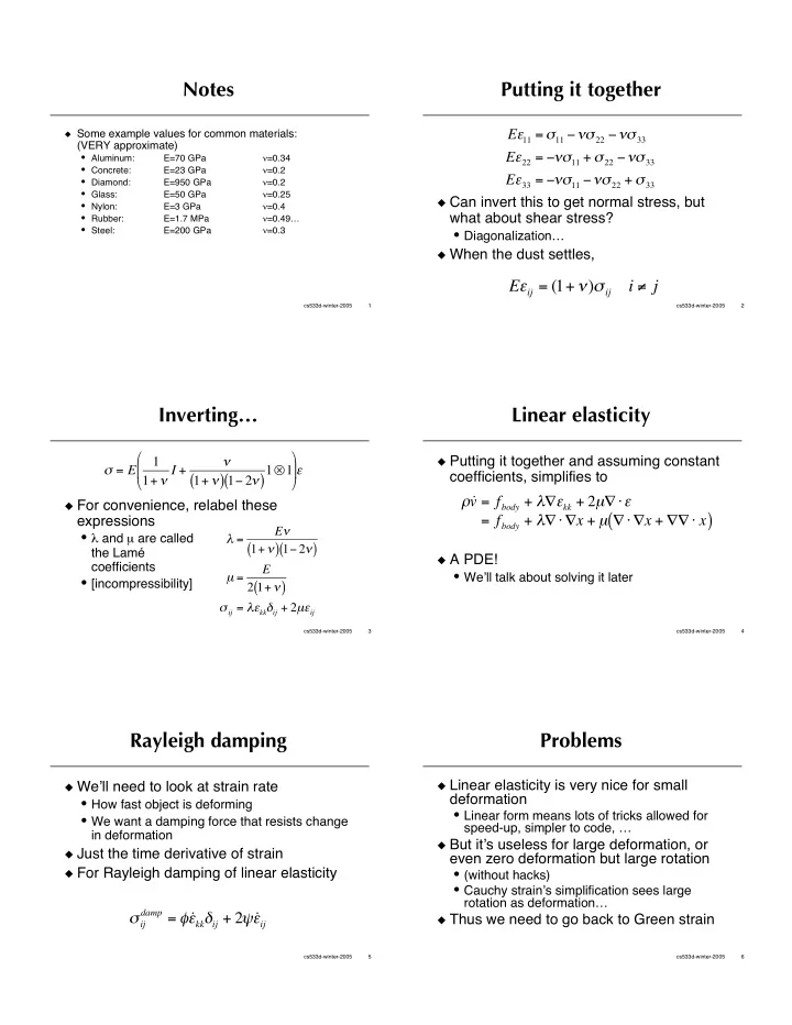
Notes

Some example values for common materials:

(VERY approximate)

• Aluminum:

E=70 GPa =0.34

• Concrete:

E=23 GPa =0.2

• Diamond:

E=950 GPa =0.2

• Glass:

E=50 GPa =0.25

• Nylon:

E=3 GPa =0.4

• Rubber:

E=1.7 MPa =0.49…

• Steel:

E=200 GPa =0.3

2 cs533d-winter-2005

Putting it together

Can invert this to get normal stress, but

what about shear stress?

• Diagonalization…

When the dust settles,

E11 = 11 22 33 E22 = 11 + 22 33 E33 = 11 22 + 33

Eij = (1+ ) ij i j

3 cs533d-winter-2005

Inverting…

For convenience, relabel these

expressions

• and µ are called

the Lamé coefficients

• [incompressibility]

= E 1 1+ I +

• 1+

( ) 1 2 ( )

11

• =

E 1+

( ) 1 2 ( )

µ = E 2 1+

( )

ij = kkij + 2µij

4 cs533d-winter-2005

Linear elasticity

Putting it together and assuming constant

coefficients, simplifies to

A PDE!

• We’ll talk about solving it later

˙ v = fbody + kk + 2µ = fbody + x + µ x + x

( )

5 cs533d-winter-2005

Rayleigh damping

We’ll need to look at strain rate

• How fast object is deforming
• We want a damping force that resists change

in deformation

Just the time derivative of strain For Rayleigh damping of linear elasticity

ij

damp = ˙

• kkij + 2˙
• ij

6 cs533d-winter-2005

Problems

Linear elasticity is very nice for small

deformation

• Linear form means lots of tricks allowed for

speed-up, simpler to code, …

But it’s useless for large deformation, or

even zero deformation but large rotation

• (without hacks)
• Cauchy strain’s simplification sees large

rotation as deformation…

Thus we need to go back to Green strain

SLIDE 2

7 cs533d-winter-2005

(Almost) Linear Elasticity

Use the same constitutive model as before,

but with Green strain tensor

This is the simplest general-purpose

elasticity model

Animation probably doesn’t need anything

more complicated

• Except perhaps for dealing with

incompressible materials

8 cs533d-winter-2005

2D Elasticity

Let’s simplify life before starting numerical

methods

The world isn’t 2D of course, but want to track

• nly deformation in the plane

Have to model why

• Plane strain: very thick material, 3•=0

[explain, derive 3•]

• Plane stress: very thin material, 3•=0

[explain, derive 3• and new law, note change in incompressibility singularity]

9 cs533d-winter-2005

Finite Volume Method

Simplest approach: finite volumes

• We picked arbitrary control volumes before
• Now pick fractions of triangles from a triangle mesh

Split each triangle into 3 parts, one for each corner E.g. Voronoi regions Be consistent with mass!

• Assume A is constant in each triangle (piecewise

linear deformation)

• [work out]
• Note that exact choice of control volumes not critical -

constant times normal integrates to zero

10 cs533d-winter-2005

Finite Element Method

#1 most popular method for elasticity problems (and

many others too)

FEM originally began with simple idea:

• Can solve idealized problems (e.g. that strain is constant over a

triangle)

• Call one of these problems an element
• Can stick together elements to get better approximation

Since then has evolved into a rigourous mathematical

algorithm, a general purpose black-box method

• Well, almost black-box…

11 cs533d-winter-2005

Modern Approach

Galerkin framework (the most common) Find vector space of functions that solution (e.g. X(p))

lives in

• E.g. bounded weak 1st derivative: H1

Say the PDE is L[X]=0 everywhere (“strong”) The “weak” statement is Y(p)L[X(p)]dp=0

for every Y in vector space

Issue: L might involve second derivatives

• E.g. one for strain, then one for div sigma
• So L, and the strong form, difficult to define for H1

Integration by parts saves the day

12 cs533d-winter-2005

Weak Momentum Equation

Ignore time derivatives - treat acceleration

as an independent quantity

• We discretize space first, then use “method of

lines”: plug in any time integrator

L X

[ ] = ˙

˙ X fbody

Y L X

[ ]

• =

Y ˙ ˙ X fbody

( )

• =

Y˙ ˙ X

• Yfbody
• Y
• =

Y˙ ˙ X

• Yfbody
• +

Y

SLIDE 3

13 cs533d-winter-2005

Making it finite

The Galerkin FEM just takes the weak equation, and

restricts the vector space to a finite-dimensional one

• E.g. Continuous piecewise linear - constant gradient over each

triangle in mesh, just like we used for Finite Volume Method

This means instead of infinitely many test functions Y to

consider, we only need to check a finite basis

The method is defined by the basis

• Very general: plug in whatever you want - polynomials, splines,

wavelets, RBF’s, …

14 cs533d-winter-2005

Linear Triangle Elements

Simplest choice Take basis {i} where

i(p)=1 at pi and 0 at all the other pj’s

• It’s a “hat” function

Then X(p)=i xii(p) is the continuous piecewise

linear function that interpolates particle positions

Similarly interpolate velocity and acceleration Plug this choice of X and an arbitrary Y= j (for

any j) into the weak form of the equation

Get a system of equations (3 eq. for each j)

15 cs533d-winter-2005

The equations

j ˙ ˙ x

ii i

• j fbody
• +

j

• = 0

ji˙ ˙ x

i

• i
• =

j fbody

• j
• Note that j is zero on all but the triangles

surrounding j, so integrals simplify

• Also: naturally split integration into separate

triangles