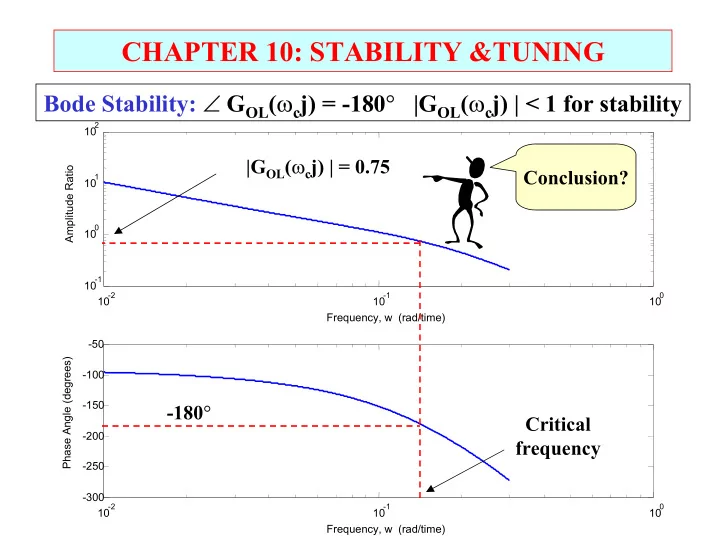
chapter 10 stability tuning
play

CHAPTER 10: STABILITY &TUNING Bode Stability: G OL ( c j) = - PowerPoint PPT Presentation

CHAPTER 10: STABILITY &TUNING Bode Stability: G OL ( c j) = -180 |G OL ( c j) | < 1 for stability 2 10 |G OL ( c j) | = 0.75 Amplitude Ratio Conclusion? 1 10 0 10 -1 10 -2 -1 0 10 10 10 Frequency, w


  1. CHAPTER 10: STABILITY &TUNING Bode Stability: ∠ G OL ( ω c j) = -180 ° |G OL ( ω c j) | < 1 for stability 2 10 |G OL ( ω c j) | = 0.75 Amplitude Ratio Conclusion? 1 10 0 10 -1 10 -2 -1 0 10 10 10 Frequency, w (rad/time) -50 Phase Angle (degrees) -100 -150 -180 ° Critical -200 frequency -250 -300 -2 -1 0 10 10 10 Frequency, w (rad/time)

  2. CHAPTER 10: STABILITY &TUNING Let’s review what we have accomplished so far. • We can evaluate the stability of a process without control by evaluating the roots of char. equation • We can evaluate the stability of a process under feedback by either - evaluating the roots of char. equation - Bode method (required for process with dead time) • These are local tests, caution about non-linearity • Stability does not guarantee good performance !!!! • Unstable system performance always poor!!!

  3. CHAPTER 10: STABILITY &TUNING 1. What else can we do with this neat technology? Tune controllers   1 ∞ d CV = + − + MV ( t ) K E ( t ) E ( t ' ) dt ' T I ∫   c d T dt F S   0 I solvent F A pure A AC Ziegler-Nichols Tuning We can tune controllers. The basic idea is to keep a “reasonable” margin from instability limit. This “reasonable” margin might give good performance.

  4. CHAPTER 10: STABILITY &TUNING 1. What else can we do with this neat technology? Tune controllers Controller Kc TI Td P-only Ku/2 --- --- PI Ku/2.2 Pu/1.2 --- PID Ku/1.7 Pu/2.0 Pu/8 • Gain margin is approximately 2 • Integral mode is required for zero s-s offset • Derivative has stabilizing effect

  5. CHAPTER 10: STABILITY &TUNING F S solvent Ziegler-Nichols tuning F A pure A • Generally, Ziegler- AC Nichols tuning is not the best initial tuning S-LOOP plots deviation variables (IAE = 23.3131) 2 method. Controlled Variable 1.5 • However, these two 1 0.5 guys were real 0 0 50 100 150 200 250 pioneers in the field! Time 150 Its taken 50 years to Manipulated Variable 100 surpass their 50 guidelines. 0 -50 0 50 100 150 200 250 Time

  6. CHAPTER 10: STABILITY &TUNING 2. What else can we do with this neat technology? Understand why detuning is required for tough processes. 10 As dead time increases, we KcKp must detune the controller. 1 0.1 0 0.2 0.4 0.6 0.8 1 fraction dead time In this plot, ( θ + τ ) is constant and θ / ( θ + τ ) Ziegler-Nichols Ciancone is changed.

  7. CHAPTER 10: STABILITY &TUNING 3. What else can we do with this neat technology? Understand need for “robustness”. After we tune the controller, we change the flow of solvent. What happens? F S solvent F S = 3.0 to 6.9 m3/min F A pure A AC

  8. CHAPTER 10: STABILITY &TUNING 3. What else can we do with this neat technology? Understand need for “robustness”. 0 10 amplitude ratio Must consider the model error when selecting controller -5 tuning 10 -2 -1 0 10 10 10 frequency (rad/time) Range of critical 0 frequencies. Smallest is most conservative phase angle -100 -180 ° -200 -300 -2 -1 0 10 10 10 frequency (rad/time)

  9. CHAPTER 10: STABILITY &TUNING 3. What else can we do with this neat technology? Understand need for “robustness”. Tune for the process response that is slowest, has highest fraction dead time, and largest process gain. This will give least aggressive controller. F S solvent F S = 3.0 to 6.9 m3/min F A pure A AC

  10. Bode calculations can be done by hand, easier with S_LOOP ************************************************************* * S_LOOP: SINGLE LOOP CONTROL SYSTEM ANALYSIS * * BODE PLOT OF GOL(s) = Gp(s)Gc(s) * * * * Characteristic Equation = 1 + GOL(s) * ************************************************************* SELECT THE APPROPRIATE MENU ITEM MODIFY... PRESENT VALUES 1) Lowest Frequency 0.01 2) Highest Frequency 0.30 3) Create Bode plot and calculate the results at critical frequency 4) Return to main menu Enter the desired selection: 2 10 ************************************************* Amplitude Ratio 1 Critical frequency and amplitude ratio 10 from Bode plot of GOL ************************************************* 0 10 Caution: 1) cross check with plot because of possible -1 10 -2 -1 0 MATLAB error in calculating the phase angle 10 10 10 Frequency, w (rad/time) 2) the program finds the first crossing of -180 -50 Phase Angle (degrees) The critical frequency is between 0.14263 -100 and 0.14287 -150 -200 The amplitude ratio at the critical frequency is 0.74797 -250 Or, write your own program in MATLAB . -300 -2 -1 0 10 10 10 Frequency, w (rad/time)

  11. CHAPTER 10: STABILITY &TUNING Match your select of tuning method to tuning goals!

  12. CHAPTER 10: TUNING & STABILITY WORKSHOP 2 Answer true or false to each of the following questions and explain each answer. A. A closed-loop system is stable only if the process and the controller are both stable. B. The Bode stability method proves that the closed- loop system is stable for only sine inputs. C. G OL (s) is the process model, G P (s), and sensor, final element, and signal transmission dynamics D. A process would be stable if it had three poles with the following values: -1, -.2, and 0.

  13. CHAPTER 10: TUNING & STABILITY WORKSHOP 3 The PID controller has been tuned for a three-tank mixer. Later, we decide to include another mixing tank in the process. If we do not retune the controller, will the control system be stable with the four-tank mixer? F S solvent F A pure A K c = 30 AC T I = 11 T d = 0.8

  14. CHAPTER 10: TUNING & STABILITY WORKSHOP 1 The data below is a process reaction curve for a process, plotted in deviation variables. Determine the tuning for a PID controller using the Ziegler-Nichols method. 4 Controlled Variable 3 2 1 v1 0 TC -1 0 5 10 15 20 25 30 35 40 45 50 Time 15 Manipulated Variable v2 10 5 0 0 5 10 15 20 25 30 35 40 45 50 Time

  15. CHAPTER 11: DIGITAL CONTROL When I complete this chapter, I want to be able to do the following. • Identify examples of analog and digital computation and signal transmission. • Program a digital PID calculation • Select a proper execution rate for a feedback controller. • Tune a digital PID

  16. CHAPTER 11: DIGITAL CONTROL Making the steam engine work all the time governor Inventors wanted to control the pressure of the boiler and the speed of the device driven by the steam (using a governor). People experienced - Explosions! - Unstable behavior And control engineering was born! http://oldenginehouse.users.btopenworld.com/watt.htm

  17. CHAPTER 11: DIGITAL CONTROL Manual Operation • Manual People know more than machines, so operation leave decisions to them. • Mechanical devices Temperature indicator • Pneumatic Should I adjust the devices valve or should I run? • Electronic devices • Digital calculations • Digital calc. & Emergency communication cooling

  18. CHAPTER 11: DIGITAL CONTROL Mechanical Device • Manual The value of the variable is represented operation by position of equipment. • Mechanical How do I change the set point? devices Location of the fulcrum • Pneumatic determines the devices ∆ gate/ ∆ level • Electronic devices Float measures • Digital Raising and calculations the liquid level lowering the gate • Digital calc. & affects the flowin communication

  19. CHAPTER 11: DIGITAL CONTROL Pneumatic Device • Manual The value of the variable is proportional operation to air pressure ( 50 - 150 C = 3 -15 psi ). • Mechanical devices How do I perform the v1 • Pneumatic PID devices TC calculation? • Electronic devices • Digital v2 calculations • Digital calc. & The signal is 3-15 psi air Air pressure moves communication pressure in a pipe. flexible diaphragm

  20. CHAPTER 11: DIGITAL CONTROL Analog computation!   t 1 d E ( t ) ∫ = + + + MV ( t ) K E ( t ) E ( t ' ) dt ' T I   c d T dt   I 0 Pneumatic Electronic From Harriott, P., Process Control, McGraw-Hill, New York, 1964

  21. CHAPTER 11: DIGITAL CONTROL Pneumatic & Electronic Devices • Manual Principle of analog computation! operation   • Mechanical t 1 d E ( t ) ∫ = + + + MV ( t ) K E ( t ) E ( t ' ) dt ' T I   devices c d T dt   I 0 • Pneumatic devices Build a physical system that (approximately) • Electronic obeys the same model. devices • Pneumatic - force balance (Newton’s laws) • Digital • Electronic - current balance (Kirkoff’s laws) calculations I wonder what these devices look like. • Digital calc. & communication

  22. CHAPTER 11: DIGITAL CONTROL Electronic Device • Manual The variable is proportional to current or operation voltage ( 50 - 150 C = 4 - 20 mA ). • Mechanical devices I’ll use analog v1 • Pneumatic computation devices TC again. • Electronic devices • Digital v2 calculations • Digital calc. & The signal is 4-20 mA Current converted to air communication transmitted by wire. pressure to affect valve

  23. CHAPTER 11: DIGITAL CONTROL Digital control employs a distributed computing network Why?

Download Presentation
Download Policy: The content available on the website is offered to you 'AS IS' for your personal information and use only. It cannot be commercialized, licensed, or distributed on other websites without prior consent from the author. To download a presentation, simply click this link. If you encounter any difficulties during the download process, it's possible that the publisher has removed the file from their server.

Recommend


More recommend