
SLIDE 1
CHAPTER 9: PID TUNING
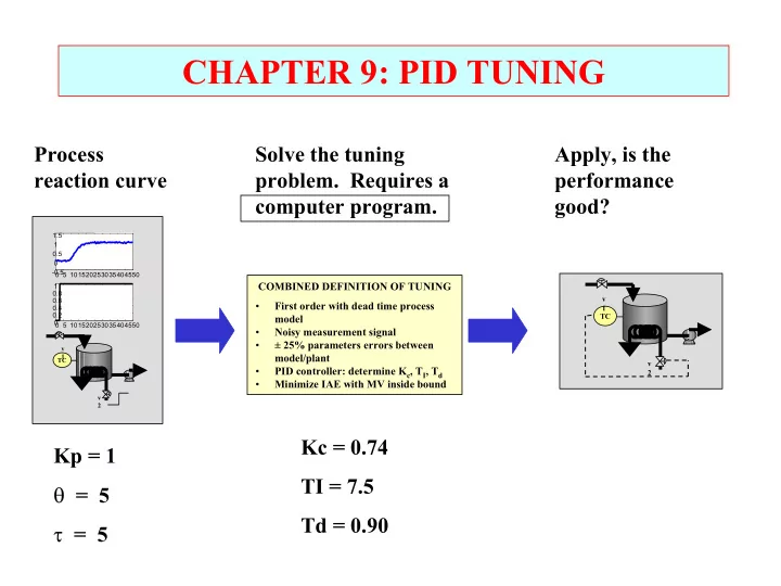
COMBINED DEFINITION OF TUNING
- First order with dead time process
model
- Noisy measurement signal
- ± 25% parameters errors between
model/plant
- PID controller: determine Kc, TI, Td
- Minimize IAE with MV inside bound
Kp = 1 θ = 5 τ = 5
TC v 1 v 2
0 5 101520253035404550
- 0.5
0.5 1 1.5 0 5 101520253035404550 0.2 0.4 0.6 0.8 1 TC v 1 v 2
Kc = 0.74 TI = 7.5 Td = 0.90 Process reaction curve Solve the tuning
- problem. Requires a
computer program. Apply, is the performance good?