CHAPTER 7: THE FEEDBACK LOOP Disturbance Response = IAE = - PowerPoint PPT Presentation

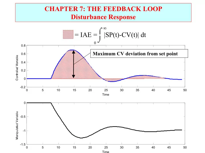
CHAPTER 7: THE FEEDBACK LOOP Disturbance Response ∞ ⌠ = IAE = |SP(t)-CV(t)| dt ⌡ 0 0.8 Maximum CV deviation from set point 0.6 0.4 0.2 0 -0.2 0 5 10 15 20 25 30 35 40 45 50 Time 0 -0.5 -1 -1.5 0 5 10 15 20 25 30 35 40 45 50 Time

CHAPTER 7: THE FEEDBACK LOOP • To reduce the variability in the CV, we increase the variability in the MV. • We must design plant with MV’s 20 Controlled Variable that can be adjusted at low cost. 10 0 -10 -20 0 100 200 300 400 500 600 700 800 900 1000 Time 20 Manipulated Variable 10 0 -10 -20 0 100 200 300 400 500 600 700 800 900 1000 Time

CHAPTER 7: THE FEEDBACK LOOP Class exercise: For each of the performance measures below, determine a good value, i.e., large/small, positive/negative, etc. • Offset • MV overshoot • IAE • Maximum CV deviation • Decay ratio • CV variance • Rise time • MV variance • Settling time Can we achieve good values for all at the same time? What are the tradeoffs?

Class exercise: Comment on the quality of control for the four responses below. S-LOOP plots deviation variables (IAE = 17.5417) S-LOOP plots deviation variables (IAE = 43.9891) 1.5 3 1 2 Controlled Variable Controlled Variable 0.5 A 1 B 0 0 -0.5 -1 0 20 40 60 80 100 120 0 20 40 60 80 100 120 Time Time 2 4 1.5 Manipulated Variable 3 Manipulated Variable 1 2 0.5 1 0 0 -0.5 0 20 40 60 80 100 120 -1 0 20 40 60 80 100 120 Time Time S-LOOP plots deviation variables (IAE = 34.2753) S-LOOP plots deviation variables (IAE = 24.0376) 1.5 1.5 Controlled Variable 1 1 Controlled Variable 0.5 0.5 C D 0 0 -0.5 -0.5 0 20 40 60 80 100 120 0 20 40 60 80 100 120 Time Time 1 1.5 Manipulated Variable 1 0.5 Manipulated Variable 0.5 0 0 -0.5 -0.5 0 20 40 60 80 100 120 0 20 40 60 80 100 120 Time Time

Class exercise: Comment on the quality of control for the four responses below. S-LOOP plots deviation variables (IAE = 17.5417) S-LOOP plots deviation variables (IAE = 43.9891) 1.5 3 1 2 Controlled Variable Controlled Variable 0.5 A 1 B 0 0 -0.5 -1 0 20 40 60 80 100 120 Generally acceptable 0 20 40 60 80 100 120 Time Too oscillatory Time 2 4 1.5 Manipulated Variable 3 Manipulated Variable 1 2 0.5 1 0 0 -0.5 0 20 40 60 80 100 120 -1 0 20 40 60 80 100 120 Time Time S-LOOP plots deviation variables (IAE = 34.2753) S-LOOP plots deviation variables (IAE = 24.0376) 1.5 1.5 Controlled Variable 1 1 Controlled Variable 0.5 0.5 C D 0 0 Gets close quickly; -0.5 -0.5 0 20 40 60 80 100 120 0 20 40 60 80 100 120 Too slow Time Time Gets to set point slowly 1 1.5 Manipulated Variable 1 0.5 Manipulated Variable 0.5 0 0 -0.5 -0.5 0 20 40 60 80 100 120 0 20 40 60 80 100 120 Time Time

CHAPTER 7: THE FEEDBACK LOOP We can apply feedback via many approaches 1, No control - The variable responds to all inputs, it “drifts”. 2. Manual - A person observes measurements and introduces changes to compensate, adjustment depends upon the person. 3. On-Off - The manipulated variable has only two states, this results in oscillations in the system. 4. Continuous, automated - This is a modulating control that has corrections related to the error from desired. 5. Emergency - This approach takes extreme action (shutdown) when a dangerous situation occurs.

CHAPTER 7: THE FEEDBACK LOOP, WORKSHOP 1 The control valve is used to introduce a variable resistance to flow. • What is the body of the valve? • Describe three bodies and what factors are important in selecting. • What is the actuator? • What power source is used? What happens when the power source fails?

CHAPTER 7: THE FEEDBACK LOOP, WORKSHOP 2 Recommend the correct failure position (open or closed) for each of the circled control valves. PI 1 AT PI 1 4 FT TI 1 PI 1 5 TI 5 TI feed 2 TI product 6 PT 1 TI 3 TI TI TI 7 9 10 TI 4 TI FT FI 8 2 TI 3 11 fuel PI PI PI air 2 3 6

CHAPTER 8: THE PID CONTROLLER When I complete this chapter, I want to be able to do the following. • Understand the strengths and weaknesses of the three modes of the PID • Determine the model of a feedback system using block diagram algebra • Establish general properties of PID feedback from the closed-loop model

CHAPTER 8: THE PID CONTROLLER Outline of the lesson. • General Features and history of PID • Model of the Process and controller - the Block Diagram • The Three Modes with features - Proportional - Integral - Derivative • Typical dynamic behavior

CHAPTER 8: THE PID CONTROLLER PROPERTIES THAT WE SEEK IN A CONTROLLER • Good Performance - feedback measures from Chapter 7 • Wide applicability - adjustable parameters v1 TC • Timely calculations - avoid convergence loops • Switch to/from manual - v2 bumplessly • Extensible - enhanced easily

CHAPTER 8: THE PID CONTROLLER SOME BACKGROUND IN THE CONTROLLER • Developed in the 1940’s, remains workhorse of practice • Not “optimal”, based on good properties of each mode v1 TC • Programmed in digital control equipment • ONE controlled variable (CV) and v2 ONE manipulated variable (MV). Many PID’s used in a plant.

CHAPTER 8: THE PID CONTROLLER Proportional MV = E SP = Set controller point Integral output + + - CV = Derivative Controlled variable Note : Error = E ≡ SP - CV sensor Final Process element variable PROCESS Three “modes”: Three ways of using the time-varying behavior of the measured variable

CHAPTER 8: THE PID CONTROLLER GENERAL CLOSED-LOOP MODEL BASED ON BLOCK DIAGRAM D(s) G d (s) SP(s) E(s) CV(s) MV(s) + + G C (s) G v (s) G P (s) + - CV m (s) G S (s) Transfer functions Variables G C (s) = controller CV(s) = controlled variable G v (s) = valve + CV m (s) = measured value of CV(s) G P (s) = feedback process D(s) = disturbance G S (s) = sensor E(s) = error G d (s) = disturbance process MV(s) = manipulated variable SP(s) = set point

CHAPTER 8: THE PID CONTROLLER D(s) G d (s) SP(s) E(s) CV(s) MV(s) + + G C (s) G v (s) G P (s) + - CV m (s) G S (s) Let’s audit • Where are the models for the transmission, and signal our conversion? understanding • What is the difference between CV(s) and CV m (s)? • What is the difference between G P (s) and G d (s)? • How do we measure the variable whose line is indicated by the red circle? • Which variables are determined by a person, which by computer?

CHAPTER 8: THE PID CONTROLLER D(s) G d (s) SP(s) E(s) CV(s) MV(s) + + G C (s) G v (s) G P (s) + - CV m (s) G S (s) Set point response Disturbance Response CV ( s ) G ( s ) G ( s ) G ( s ) G ( s ) CV ( s ) = 1 d p v c = 1 + D ( s ) G ( s ) G ( s ) G ( s ) G ( s ) + SP ( s ) G ( s ) G ( s ) G ( s ) G ( s ) p v c S p v c S • Which elements in the control system affect system stability? • Which elements affect dynamic response?

Proportional MV SP E CHAPTER 8: + Integral + CV - Derivative THE PID CONTROLLER, Note : Error = E ≡ SP - CV The Proportional Mode PROCESS “correction proportional to error.” = + Time domain : MV ( t ) K E ( t ) I c p MV ( s ) = = Transfer function : G ( s ) K C C E ( s ) How does this differ from K C = controller gain the process gain, K p ?

Proportional MV SP E CHAPTER 8: + Integral + CV - Derivative THE PID CONTROLLER, Note : Error = E ≡ SP - CV The Proportional Mode PROCESS “correction proportional to error.” = + Time domain : MV ( t ) K E ( t ) I c p K p depends upon the process (e.g., reactor volume, flows, temperatures, etc.) K C = controller gain K C is a number we select; it is used in the computer each time the How does this differ from controller equation is calculated the process gain, K p ?

Proportional MV SP E CHAPTER 8: + Integral + CV - Derivative THE PID CONTROLLER, Note : Error = E ≡ SP - CV The Proportional Mode PROCESS = + Time domain : MV ( t ) K E ( t ) I c p

Proportional MV SP E CHAPTER 8: + Integral + CV - Derivative THE PID CONTROLLER, Note : Error = E ≡ SP - CV The Proportional Mode PROCESS Key feature of closed-loop performance with P-only Final value ∆ ∆ D K D K = = ≠ d d CV ( t ) lim s 0 after → ∞ + + t s 1 K K 1 K K → s 0 disturbance: c p c p • We do not achieve zero offset; don’t return to set point ! • How can we get very close by changing a controller parameter? • Any possible problems with suggestion?