Applications of 2 nd -order ODEs: Mechanical & Electrical - - PowerPoint PPT Presentation

Applications of 2nd-order ODEs:

Mechanical & Electrical Vibrations

• There are two important areas of application for second
• rder linear equations with constant coefficients, which are

in modeling mechanical and electrical oscillations.

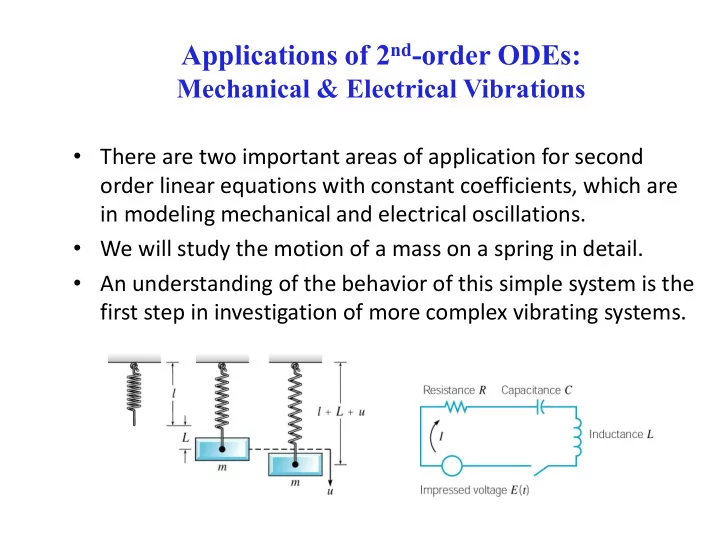
• We will study the motion of a mass on a spring in detail.
• An understanding of the behavior of this simple system is the

first step in investigation of more complex vibrating systems.

Spring – Mass System

• Suppose a mass m hangs from a vertical spring of original

length l. The mass causes an elongation L of the spring.

• The force FG of gravity pulls the mass down. This force has

magnitude mg, where g is acceleration due to gravity.

• The force FS of the spring stiffness pulls the mass up. For

small elongations L, this force is proportional to L. That is, Fs = kL (Hooke’s Law).

• When the mass is in equilibrium, the forces balance each
• ther:

kL mg 

Spring Model

• We will study the motion of a mass when it is acted on by an

external force (forcing function) and/or is initially displaced.

• Let u(t) denote the displacement of the mass from its

equilibrium position at time t, measured downward.

• Let f be the net force acting on the mass. We will use

Newton’s 2nd Law:

• In determining f, there are four separate forces to consider:

– Weight: w = mg (downward force) – Spring force: Fs = - k(L+ u) (up or down force, see next slide) – Damping force: Fd(t) = -  u (t) (up or down, see following slide) – External force: F(t) (up or down force, see text)

) ( ) ( t f t u m   

Spring Model: Spring Force Details

• The spring force Fs acts to restore a spring to the natural

position, and is proportional to L + u. If L + u > 0, then the spring is extended and the spring force acts upward. In this case

• If L + u < 0, then spring is compressed a distance of |L + u|,

and the spring force acts downward. In this case

• In either case,

) ( u L k Fs   

     

u L k u L k u L k Fs         ) ( u L k Fs   

Spring Model: Damping Force Details

• The damping or resistive force Fd acts in the opposite direction as

the motion of the mass. This can be complicated to model. Fd may be due to air resistance, internal energy dissipation due to action

• f spring, friction between the mass and guides, or a mechanical

device (dashpot) imparting a resistive force to the mass.

• We simplify this and assume Fd is proportional to the velocity.
• In particular, we find that

– If u > 0, then u is increasing, so the mass is moving downward. Thus Fd acts upward and hence Fd = -  u, where  > 0. – If u < 0, then u is decreasing, so the mass is moving upward. Thus Fd acts downward and hence Fd = -  u ,  > 0.

• In either case,

), ( ) (       t u t Fd

Spring Model: Differential Equation

• Taking into account these forces, Newton’s Law becomes:
• Recalling that mg = kL, this equation reduces to

where the constants m, , and k are positive.

• We can prescribe initial conditions also:
• It follows from Theorem 3.2.1 that there is a unique solution to

this initial value problem. Physically, if the mass is set in motion with a given initial displacement and velocity, then its position is uniquely determined at all future times.

 

) ( ) ( ) ( ) ( ) ( ) ( ) ( t F t u t u L k mg t F t F t F mg t u m

d s

             ) ( ) ( ) ( ) ( t F t ku t u t u m       

) ( , ) ( v u u u   

Example 1: Find Coefficients (1 of 2)

• A 4 lb mass stretches a spring 2". The mass is displaced an

additional 6" and then released; and is in a medium that exerts a viscous resistance of 6 lb when the mass has a velocity of 3 ft/sec. Formulate the IVP that governs the motion of this mass:

• Find m:
• Find  :
• Find k:

ft sec lb 8 1 sec / ft 32 lb 4

2 2

       m m g w m mg w

ft sec lb 2 sec / ft 3 lb 6 lb 6          u ft lb 24 ft 6 / 1 lb 4 in 2 lb 4         k k k L k Fs

) ( , ) ( ), ( ) ( ) ( ) ( v u u u t F t ku t u t u m          

Example 1: Find IVP (2 of 2)

• Thus our differential equation becomes

and hence the initial value problem can be written as

• This problem can be solved using the

methods of Chapter 3.3 and yields the solution

) ( 24 ) ( 2 ) ( 8 1       t u t u t u ) ( , 2 1 ) ( ) ( 192 ) ( 16 ) (          u u t u t u t u

)) 2 8 sin( 2 ) 2 8 cos( 2 ( 4 1 ) (

8

t t e t u

t

 



0.2 0.4 0.6 0.8 t 0.2 0.2 0.4 0.6 0.8 u t

)) 2 8 sin( 2 ) 2 8 cos( 2 ( 4 1 ) (

8

t t e t u

t

 



Spring Model: Undamped Free Vibrations (1 of 4)

• Recall our differential equation for spring motion:
• Suppose there is no external driving force and no damping.

Then F(t) = 0 and  = 0, and our equation becomes

• The general solution to this equation is

) ( ) (     t ku t u m

) ( ) ( ) ( ) ( t F t ku t u t u m        m k t B t A t u / where , sin cos ) (

2

     

Spring Model: Undamped Free Vibrations (2 of 4)

• Using trigonometric identities, the solution

can be rewritten as follows: where

• Note that in finding , we must be careful to choose the

correct quadrant. This is done using the signs of cos and sin. m k t B t A t u / , sin cos ) (

2

     

 

, sin sin cos cos ) ( cos ) ( sin cos ) ( t R t R t u t R t u t B t A t u                

A B B A R R B R A          tan , sin , cos

2 2

Spring Model: Undamped Free Vibrations (3 of 4)

• Thus our solution is

where

• The solution is a shifted cosine (or sine) curve, that describes simple

harmonic motion, with period

• The circular frequency 0 (radians/time) is the natural frequency of

the vibration, R is the amplitude of the maximum displacement of mass from equilibrium, and  is the phase or phase angle (dimensionless).

 

        t R t B t A t u cos sin cos ) (

k m T    2 2   m k /

0 



Spring Model: Undamped Free Vibrations (4 of 4)

• Note that our solution

is a shifted cosine (or sine) curve with period

• Initial conditions determine A & B, hence also the amplitude R.
• The system always vibrates with the same frequency 0 ,

regardless of the initial conditions.

• The period T increases as m increases, so larger masses vibrate

more slowly. However, T decreases as k increases, so stiffer springs cause a system to vibrate more rapidly.

 

m k t R t B t A t u / , cos sin cos ) (          

k m T  2 

Example 2: Find IVP (1 of 3)

• A 10 lb mass stretches a spring 2". The mass is displaced an

additional 2" and then set in motion with an initial upward velocity of 1 ft/sec. Determine the position of the mass at any later time, and find the period, amplitude, and phase of the motion.

• Find m:
• Find k:
• Thus our IVP is

ft sec lb 16 5 sec / ft 32 lb 10

2 2

       m m g w m mg w ft lb 60 ft 6 / 1 lb 10 in 2 lb 10         k k k L k Fs

1 ) ( , 6 / 1 ) ( , ) ( 60 ) ( 16 / 5         t u u t u t u

) ( , ) ( , ) ( ) ( v u u u t ku t u m       

Example 2: Find Solution (2 of 3)

• Simplifying, we obtain
• To solve, use methods of Ch 3.3 to obtain
• r

1 ) ( , 6 / 1 ) ( , ) ( 192 ) (         u u t u t u t t t u 192 sin 192 1 192 cos 6 1 ) (   t t t u 3 8 sin 3 8 1 3 8 cos 6 1 ) (  

Example 2: Find Period, Amplitude, Phase (3 of 3)

• The natural frequency is
• The period is
• The amplitude is
• Next, determine the phase :

t t t u 3 8 sin 3 8 1 3 8 cos 6 1 ) (  

rad/sec 856 . 13 3 8 192 /     m k  sec 45345 . / 2

0 

   T ft 18162 .

2 2

   B A R

rad 40864 . 4 3 tan 4 3 tan tan

1

                



   A B

A B R B R A / tan , sin , cos      

 

409 . 3 8 cos 182 . ) ( Thus   t t u

Spring Model: Damped Free Vibrations (1 of 8)

• Suppose there is damping but no external driving force F(t):
• What is effect of the damping coefficient  on system?
• The characteristic equation is
• Three cases for the solution:

) ( ) ( ) (       t ku t u t u m 

             

2 2 2 1

4 1 1 2 2 4 ,     mk m m mk r r

   

term. damping the from expected as , ) ( lim cases, three all In : Note . 2 4 , sin cos ) ( : 4 ; 2 / where , ) ( : 4 ; , where , ) ( : 4

2 2 / 2 2 / 2 2 1 2

2 1

                  

   

t u m mk t B t A e t u mk m e Bt A t u mk r r Be Ae t u mk

t m t m t t r t r

       

 

Damped Free Vibrations: Small Damping (2 of 8)

• Of the cases for solution form, the last is most important,

which occurs when the damping is small:

• We examine this last case. Recall
• Then

and hence (damped oscillation)    

, sin cos ) ( : 4 2 / , ) ( : 4 , , ) ( : 4

2 / 2 2 / 2 2 1 2

2 1

               

 

      

 

t B t A e t u mk m e Bt A t u mk r r Be Ae t u mk

m t m t t r t r

  sin , cos R B R A  

 

 



 



t e R t u

m t

cos ) (

2 / m t

e R t u

2 /

) (

 



Damped Free Vibrations: Quasi Frequency (3 of 8)

• Thus we have damped oscillations:
• The amplitude R depends on the initial conditions, since
• Although the motion is not periodic, the parameter 

determines the mass oscillation frequency.

• Thus  is called the quasi frequency.
• Recall

 

   



sin , cos , sin cos ) (

2 /

R B R A t B t A e t u

m t

   



 

m t m t

e R t u t e R t u

2 / 2 /

) ( cos ) (

 

 

 

   

m mk 2 4

2

   

Damped Free Vibrations: Quasi Period (4 of 8)

• Compare  with 0 , the frequency of undamped motion:
• Thus, small damping reduces oscillation frequency slightly.
• Similarly, the quasi period is defined as Td = 2/. Then
• Thus, small damping increases quasi period.

km km m k km km km km m k m km m k m km 8 1 8 1 64 4 1 4 1 4 4 / 4 4 / 2 4

2 2 2 2 2 4 2 2 2 2 2 2

                                

For small 

km km km T Td 8 1 8 1 4 1 / 2 / 2

2 1 2 2 / 1 2

                                

 

Damped Free Vibrations: Neglecting Damping for Small  2/4km

(5 of 8)

• Consider again the comparisons between damped and

undamped frequency and period:

• Thus it turns out that a small  is not as telling as a small

ratio  2/4km.

• For small  2/4km, we can neglect the effect of damping

when calculating the quasi frequency and quasi period of

• motion. But if we want a detailed description of the motion
• f the mass, then we cannot neglect the damping force, no

matter how small it is.

2 / 1 2 2 / 1 2

4 1 , 4 1



                    km T T km

d

   

Damped Free Vibrations: Frequency, Period

(6 of 8)

• Ratios of damped and undamped frequency, period:
• Thus
• The importance of the relationship between 2 and 4km is

supported by our previous equations:

2 / 1 2 2 / 1 2

4 1 , 4 1



                    km T T km

d

   

  

  d km km

T

2 2

lim and lim

 



   

, sin cos ) ( : 4 2 / , ) ( : 4 , , ) ( : 4

2 / 2 2 / 2 2 1 2

2 1

               

 

      

 

t B t A e t u mk m e Bt A t u mk r r Be Ae t u mk

m t m t t r t r

Damped Free Vibrations: Critical Damping Value (7 of 8)

• Thus the nature of the solution changes as  passes through

the value

• This value of  is known as the critical damping value, and

for larger values of  the motion is said to be overdamped.

• Thus for the solutions given by these cases,

we see that the mass creeps back to its equilibrium position for solutions (1) and (2), but does not oscillate about it, as it does for small  in solution (3).

• Soln (1) is overdamped and soln (2) is critically damped.

. 2 km

   

) 3 ( , sin cos ) ( : 4 ) 2 ( 2 / , ) ( : 4 ) 1 ( , , ) ( : 4

2 / 2 2 / 2 2 1 2

2 1

               

 

      

 

t B t A e t u mk m e Bt A t u mk r r Be Ae t u mk

m t m t t r t r

Damped Free Vibrations: Characterization of Vibration (8 of 8)

• The mass creeps back to the equilibrium position for

solutions (1) & (2), but does not oscillate about it, as it does for small  in solution (3).

• Solution (1) is overdamped and
• Solution (2) is critically damped.
• Solution (3) is underdamped

   

) 3 ( (Blue) sin cos ) ( : 4 ) 2 ( Black) (Red, 2 / , ) ( : 4 ) 1 ( (Green) , , ) ( : 4

2 / 2 2 / 2 2 1 2

2 1

t B t A e t u mk m e Bt A t u mk r r Be Ae t u mk

m t m t t r t r

     

 

              

 

Example 3: Initial Value Problem (1 of 4)

• Suppose that the motion of a spring-mass system is governed by

the initial value problem

• Find the following:

(a) quasi frequency and quasi period; (b) time at which mass passes through equilibrium position; (c) time  such that |u(t)| < 0.1 for all t > .

• For Part (a), using methods of this chapter we obtain:

where

) ( , 2 ) ( , 125 .          u u u u u

                   

 

 t e t t e t u

t t

16 255 cos 255 32 16 255 sin 255 2 16 255 cos 2 ) (

16 / 16 /

) sin , cos (recall 06254 . 255 1 tan     R B R A     

Example 3: Quasi Frequency & Period (2 of 4)

• The solution to the initial value problem is:
• The graph of this solution, along with solution to the

corresponding undamped problem, is given below.

• The quasi frequency is

and quasi period is

• For the undamped case:

                   

 

 t e t t e t u

t t

16 255 cos 255 32 16 255 sin 255 2 16 255 cos 2 ) (

16 / 16 /

998 . 16 / 255   

295 . 6 / 2    

d

T

283 . 6 2 , 1      T

Example 3: Quasi Frequency & Period (3 of 4)

• The damping coefficient is  = 0.125 = 1/8, and this is 1/16 of

the critical value

• Thus damping is small relative to mass and spring stiffness.

Nevertheless the oscillation amplitude diminishes quickly.

• Using a solver, we find that |u(t)| < 0.1 for t >   47.515 sec

2 2  km

Example 3: Quasi Frequency & Period (4 of 4)

• To find the time at which the mass first passes through the

equilibrium position, we must solve

• Or more simply, solve

16 255 cos 255 32 ) (

16 /

          



 t e t u

t

sec 637 . 1 2 255 16 2 16 255                 t t

Electric Circuits

• The flow of current in certain basic electrical circuits is

modeled by second order linear ODEs with constant coefficients:

• It is interesting that the flow of current in this circuit is

mathematically equivalent to motion of spring-mass system.

• For more details, see text.

) ( , ) ( ) ( ) ( 1 ) ( ) ( I I I I t E t I C t I R t I L           